Generative Adversarial Networks

In this post, we will see how GANs have disrupted every domain and what makes GANs so powerful.

All the codes implemented in Jupyter notebook in Keras, PyTorch and Fastai.

All codes can be run on Google Colab (link provided in notebook).

Hey yo, but how?

Well sit tight and buckle up. I will go through everything in-detail.

Feel free to jump anywhere,

Introduction to GAN
Recap
Different types of GANs
- Images
  - DCGAN
  - WGAN
  - Pix2Pix
  - CycleGAN
  - ProGAN
  - StyleGAN
  - BigGAN
  - GAN semi-supervised learning
- Speech
  - GanSynth
- Text
  - MaskGAN
- Videos
Problems in GANs
Will GANs Rule the World?
- Images
- Speech
- Videos
Special Mentions
Further Reading
Footnotes and Credits

Introduction to GAN

A long time ago in a galaxy far, far away….

I-know-everything: In our last post, we saw how we can use Adversarial Machine Learning in context of security. We discussed how adversaries can abuse the model and produce malicious results which can have serious consequences in real world. The name “Adversarial” has different meaning depending on the context. In the previous post we used Adversarial Training where neural network is used to correctly classify adversarial examples by training the network on adversarial examples. In context of RL, “self play” can be seen as Adversarial Training where the network learns to play with itself. In our today’s topic which is GAN i.e. Generative Adversarial Networks, we will use Adversarial Training where a model is trained on the inputs produced by adversary. Now if there is no more gossips about the name “Adversarial”, let’s get back to the revolutionary GANs. As all posts on GANs starts with the quote from Yann LeCunn,

“The most important one, in my opinion, is adversarial training (also called GAN for Generative Adversarial Networks). This is an idea that was originally proposed by Ian Goodfellow when he was a student with Yoshua Bengio at the University of Montreal (he since moved to Google Brain and recently to OpenAI).This, and the variations that are now being proposed is the most interesting idea in the last 10 years in ML, in my opinion.” #Tradition#not#broken.

I-know-nothing: Holding up the tradition, what are GANs? Specifically, what does generative mean?

I-know-everything: Consider the example where are we are teaching a model to distinguish between dog(y=0) and cat(y=1). The traditional machine learning classification algorithms like logistic regression or perceptron algorithm tries is to find a straight line - a decision boundary - such that when a test image of dog is passed, model checks on which side of decision boundary does it falls and gives predictions accordingly. This is what we have learned from our past journey nothing new so far. But consider a different approach. Instead of learning a decision boundary, what if network learns a model of dog by looking at lot many different images of dog and same with cat, a different model of what a cat looks like. Now, when we pass a test image of dog to classify, the test image is matched against the model of dog and model of cat to make prediction. It’s simply opposite approach, instead of using features for predicting what class it belongs we predict the features from given image. These features will tell us how close it resembles to a dog or cat. Algorithms like logistic regression and perceptron learns mappings directly from space of inputs \(\chi\) to labels {0, 1} i.e. p(y \(\vert\) x) where y \(\in\) {0, 1} and these are called discriminative learning algorithms. Now, instead of learning the mapping from input space, what if model learns the distribution of input features? This is the idea behind generative learning algorithms. They learn p(x \(\vert\) y), for example, if y=0 indicates it’s a dog then p(x \(\vert\) y=0) models the distribution of dog’s features and p(x \(\vert\) y=1) modeling the distribution of cat’s features. GANs belong to the family of generative models. This means that GANs samples data from training set, a distribution \(p_{data}\), and learns to represent an estimate of that distribution, resulting in probability distribution \(p_{model}\). There are cases where GAN estimates \(p_{model}\) explicitly and in other cases model is only able to generate samples from \(p_{model}\). GAN primarily focuses on the second case generating samples from the model distribution although it is possible to design GANs that can do both.

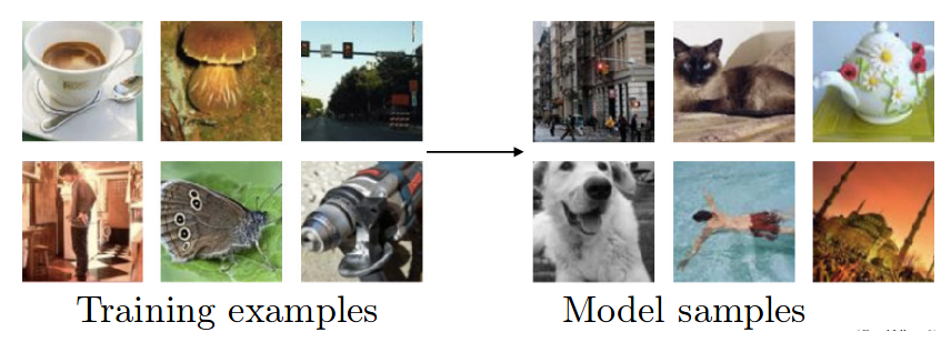
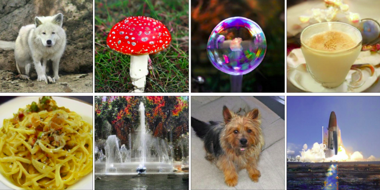
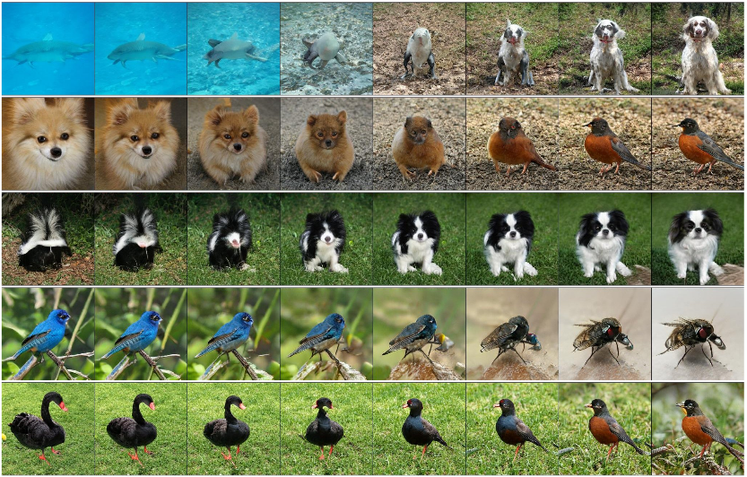
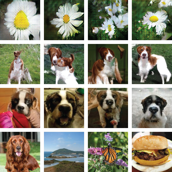
Here is an example where an ideal generative model would be able to train on examples shown on left and then create more examples from the same distribution as shown on the right.

I-know-nothing: Discriminative learning are fairly straight forward, we get data and labels and we train and get state-of-the-art results. I wonder how generative models are trained and why have they not yet been used as first go-to models?

I-know-everything: The information we gained from above discussion about generative models is that they are about comparing \(p_{model}\) which is data distribution learned by model with \(p_{data}\) which is true data distribution. Let’s see an example.

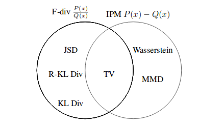
In the example above, the blue region shows the true data distribution (\(p_{data}\)), where black dot represents each image in dataset. Now our model, a neural network in yellow draws points from unit Gaussian, red in color, and generates a distribution as shown in green color which is the distribution learned by model (\(p_{model}\) or \(\hat{p}_{\theta}\)). Our goal then is find parameters \(\theta\) of model that produce a distribution that closely matches the true data distribution. Therefore, you can imagine the green distribution starting out random and then the training process iteratively changing the parameters \(\theta\) to stretch and squeeze it to better match the blue distribution. There are many loss function –as in case of supervised learning– which deal with comparing two distribution such as Kullback-Liebler (KL) divergence, Reverse-KL divergence and Jenson-Shannon Divergence (JSD). These belong to F-divergence class of probability distance metrics. The other class is Integral Probability Metrics (IPMs). For the IPMS, we have the Wassterstein distance(which is used in the WGAN) and the Maximum Mean Discrepancy (MMD). Difference between F-divergence and IPMs is F-divergences determine distance using division of two probability distributions, \(\frac{P(x)}{Q(x)}\) and IPMs use the difference, P(x) - Q(x).

Most generative models like GAN, Autoregressive models or VAE have this basic setup, but differ in the details. GANs and Divergence Minimization blog by Colin explains F-divergence class using amazing visualizations.

I-know-nothing: The approach taken by GANs is certainly new when compared to previous approaches of supervised learning. I wonder in what bucket of learning does GAN go in? What’s so special about them? What learning function do they use if any?

I-know-everything: Here’s a interesting thing, they belong to both buckets of supervised learning and unsupervised learning. The GAN sets up a supervised learning problem in order to do unsupervised learning. You will understand why so once when we introduce different parts of GAN. Let’s do that! The basic idea of GAN is setting up a game between two players. The two players are generator and discriminator. The generator creates samples that are intended to come from the same distribution as the training set. The discriminator examines the samples to determine whether they are real or fake (Are the input samples similar to that in training set or not?)

So, what is the game between the two players? The generator is trained to fool the discriminator i.e. generator generates a sample and passes it to discriminator. The discriminator using traditional supervised learning is trained to classify the input sample in two classes (real or fake), fooling the discriminator means that discriminator will classify the sample generated by generator to be real instead of fake. And this is where the name “Adversarial” in GAN comes from (They are both adversaries of each other 😛). Here we see that generator wants to be good at fooling discriminator and discriminator wants to be good at classifying samples correctly. This fight scenario corresponds to Nash Equilibrium from Game Theory. Borrowing example of Alice and Bob from Wikipedia, Alice and Bob are in Nash equilibrium if Alice is making the best decision she can, taking into account Bob’s decision while his decision remains unchanged, and Bob is making the best decision he can, taking into account Alice’s decision while her decision remains unchanged. Likewise, a group of players are in Nash equilibrium if each one is making the best decision possible, taking into account the decisions of the others in the game as long as the other parties’ decisions remain unchanged. GAN requires finding the Nash Equilibrium of the game, which is more difficult than optimizing an objective function as done in traditional machine learning.

Okay, let’s try to understand this notion of game through more examples. Suppose the generator to be a counterfeiter, trying to make fake money, and the discriminator as being like police, trying to allow legitimate money and catch counterfeit money. To succeed in this game, the counterfeiter must learn to make money that is indistinguishable from genuine money. Another example, where the generator is person signing cheques using fake signatures and the discriminator is a bank person, trying to identify if the signature is authentic or not. To succeed in passing the cheque, the person needs to produce signature very real to the original such that bank person gets conned into thinking that fake signature is authentic. You get it right?

Now let’s dive in-detail into generator and discriminator.

GAN Framework

Discriminator(D) is a differentiable function, usually a neural network with parameter \(\theta^{(D)}\). Discriminative network which takes in input, \(\mathbf{x}\) “real sample” which comes from training set or output from generator G(\(\mathbf{z}\)) “fake sample”. The goal of discriminator is to classify the input from training set as real and the one from generator as fake. Discriminator is shown half of inputs which are real and remaining half as fakes generated by G.
Generator(G) is also differential function, another neural network with parameter \(\theta^{(G)}\). Generative network takes in input \(\mathbf{z}\), where \(\mathbf{z}\) is sample from some prior distribution, G(\(\mathbf{z}\)) yields a sample \(\mathbf{x}\) drawn from \(p_{model}\). The goal of generator is to fool discriminator.

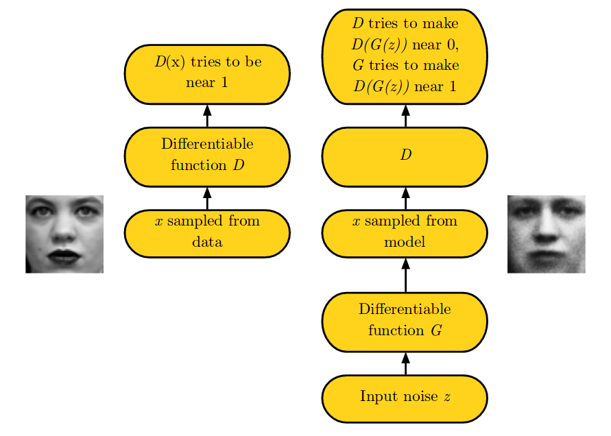
Here is the game which is played in two scenarios. In first scenario left side of the figure, training examples \(\mathbf{x}\) are randomly sampled from training dataset and used as input for first player, the discriminator(D). The goal of discriminator(D) is to output the probability that its input is real rather than fake. In first scenario, D(\(\mathbf{x}\)) tries to be near 1, classifying it to be a real. In second scenario, the inputs \(\mathbf{z}\) to the generator(G) are sampled from model’s prior over latent variables. The discriminator then receives the output from generator(G), G(\(\mathbf{z}\)) a fake sample generated by generator(G). Here, the discriminator(D) tries to make D(G(\(\mathbf{z}\))) near 0, as it is fake sample and generator(G) tries to make D(G(\(\mathbf{z}\))) near 1 to fool discriminator in classifying the fake sample as real. If both models have sufficient capacity, then the Nash equilibrium of this game corresponds to the G(\(\mathbf{z}\)) being drawn from the same distribution as the training data, and D(\(\mathbf{x}\)) = \(\frac{1}{2}\) for all \(\mathbf{x}\). How? We will prove this shortly.

Cost Functions

Above, we mentioned that GAN sets up a supervised learning problem in order to do unsupervised learning. Here is where we will see how that is true.

Discriminator’s Cost

The discriminative network is a classifier which takes in an input and classifies it to be fake or real i.e. 0 or 1. We have seen these types of problems in supervised learning which go by name binary classifiers. The output of neural network is binary which is obtained by adding sigmoid as last classification layer. As with all supervised algorithms, we require objective function to minimize. We also know that there is a particular loss function which corresponds to binary classification, binary cross entropy(BCE). The cost function used for discriminator(D) is \(J^{(D)}\)(\(\theta^{(D)}\), \(\theta^{(G)}\)), for parameters \(\theta^{(D)}\) of discriminative network and \(\theta^{(G)}\) of generative network.

We will first define cost function for one data point (\(\mathbf{x}_{1}\), \(\mathbf{y}_{1}\)) and then generalize over entire dataset for N elements.

\[\begin{aligned} J^{(D)}(\theta^{(D)}, \theta^{(G)}) &= -\mathbf{y}_{1}\log_{}D(\mathbf{x}_{1})-(1-\mathbf{y}_{1})(1-D(\mathbf{x}_{1})) \\ &= -\sum_{i=1}^{N}\mathbf{y}_{i}\log_{}D(\mathbf{x}_{i})-\sum_{i=1}^{N}(1-\mathbf{y}_{i})(1-D(\mathbf{x}_{i})) \end{aligned}\]

In GANs, \(x_{i}\) either come two sources: either \(x_{i}\) \(\sim\) \(p_{data}\), the true distribution, or \(x_{i}\) = G(\(\mathbf{z}\)) where \(\mathbf{z}\) \(\sim\) \(p_{model}\), the generator’s distribution, \(\mathbf{z}\) is sample drawn from some prior distribution. Discriminator sees exactly half of the data coming from each source i.e. half samples are real and remaining half are fake.

\[\begin{aligned} J^{(D)}(\theta^{(D)}, \theta^{(G)}) &= -\frac{1}{2} \mathbb{E}_{\mathbf{x} \sim p_{data}(\mathbf{x})}\log_{}D(\mathbf{x}) -\frac{1}{2} \mathbb{E}_{\mathbf{z} \sim p_{z}(\mathbf{z})}\log_{}(1-D(G(\mathbf{z}))) \end{aligned}\]

Minmax

To play the game, we need to complete generator’s cost function \(J^{(G)}\) too. We assume that we are playing the simplest zero-sum game, where the sum of all player’s cost is zero. In this zero-sum game, we get \(J^{(D)}\) + \(J^{(G)}\) = 0. This gives us \(J^{(G)}\) = - \(J^{(D)}\).

From looking at the equations above for \(J^{(D)}(\theta^{(D)}, \theta^{(G)})\) and figure explaining two scenarios of game, the discriminator decision are accurate when it correctly classifies fake and real samples. In terms of cost function, in first scenario with real samples, D(\(\mathbf{x}\)) tries to be near 1, i.e. maximize \(\mathbb{E}_{\mathbf{x} \sim p_{data}}[D(\mathbf{x})]\). When D(\(\mathbf{x}\)) becomes close to 1, \(\mathbb{E}[\log_{}(D(\mathbf{x}))]\) becomes close to 0 and when D(\(\mathbf{x}\)) tries to be near 0, \(\mathbb{E}[\log_{}(D(\mathbf{x}))]\) becomes close to \(-\infty\). In second scenario with fake samples, D(G(\(\mathbf{x}\))) tries to be near 0, i.e. maximize \(\mathbb{E}_{\mathbf{z}}[\log_{}(1-D(G(\mathbf{z})))]\). (Question: Show that in the limit, the maximum of the discriminator objective above is the Jenson-Shannon divergence, up to scaling and constant factors.)

The generator on other hand is trained to increase the chances of D producing a high probability i.e. 1, to classify it as real for a fake example, i.e. maximizing \(\mathbb{E}_{\mathbf{z}}[D(G(\mathbf{z}))]\) or to minimize \(\mathbb{E}_{\mathbf{z}}[1-D(G(\mathbf{z}))]\), the part of cost function (\(\mathbb{E}_{\mathbf{x} \sim p_{data}}[D(\mathbf{x})]\)) which deals with real samples will have no effect on generator as it is not sampled from generator.

So, combining both the conclusions from above, to maximize the cost function for D and minimze the second part of cost function for G, G and D are essentially playing minmax game.

We substitute V(D, G) = - \(J^{(D)}(\theta^{(D)}, \theta^{(G)})\) in cost function to get the minmax of value function as follows,

\[\begin{aligned} \min_{G} \max_{D} V(D, G) &= \mathbb{E}_{\mathbf{x} \sim p_{data}(\mathbf{x})}[\log_{}D(\mathbf{x})]+ \mathbb{E}_{\mathbf{z} \sim p_{z}(\mathbf{z})}[\log_{}(1-D(G(\mathbf{z})))] \end{aligned}\]

It’s like generator and discriminator are fighting each other on who will win. Each wants to succeed in completing it’s own objective. This game continues till we get a state, in which each model becomes an expert on what it is doing, the generative model increases its ability to get the actual data distribution and produces data similar to it, and the discriminative becomes expert in identifying the real samples. The discriminator tries to maximize tweaking only it’s parameter and G tries to minimize tweaking only it’s parameters. How amazing? And this setup helps G to produce jaw-dropping images. Can it get any better than this? (Question: Will doing maxmin produce same results?)

Another way to look at above cost function is, we require D that correctly classifies real samples x, where \(\mathbf{x} \sim p_{data}(\mathbf{x})\), hence \(\mathbb{E}_{\mathbf{x} \sim p_{data}(\mathbf{x})}[\log_{}D(\mathbf{x})]\). Maximizing this term corresponds to D being able to predict when \(\mathbf{x} \sim p_{data}(\mathbf{x})\). This is the first term of value function. Next term G fooling D in passing generated sample z, where \(\mathbf{z} \sim p_{z}(\mathbf{z})\) as real samples, hence \(\mathbb{E}_{\mathbf{z} \sim p_{z}(\mathbf{z})}[\log_{}(1-D(G(\mathbf{z})))]\). Maximizing this term means \(D(G(\mathbf{z})) \approx 0\) implying G is NOT fooling D, therefore minimize \(-D(G(\mathbf{z}))\). This again confirms the above minmax game between D and G where optimal D is maximizing the above equation and optimal G is minimizing the above equation.

On a sad note, the cost used for the generator in the minimax game is useful for theoretical analysis, but does not perform especially well in practice. This is unfortunate for the generator, because when the discriminator successfully rejects generator samples with high confidence producing a perfect discriminator, the generator’s gradient vanishes, it will produce zero everywhere, leading to vanishing gradient problem. This is main problem in training GANs called “mode collapse”.

To solve this problem, one approach is to continue to use cross-entropy minimization for the generator. Instead of flipping the sign on the discriminator’s cost to obtain a cost for the generator, we flip the target used to construct the cross-entropy cost. The cost for the generator then becomes:

\[\begin{aligned} J^{(G)} &= -\frac{1}{2} \mathbb{E}_{\mathbf{z}}\log_{}(1-D(G(\mathbf{z}))) \end{aligned}\]

Also, maximum likelihood can be used as cost function for generator,

\[\begin{aligned} J^{(G)} &= -\frac{1}{2} \mathbb{E}_{\mathbf{z}}\exp({\sigma^{-1}(D(G(\mathbf{z})))}) \end{aligned}\]

Different adversarial loss functions such as feature matching, minibatch discrimination, etc produces good results in GANs. Many such adversarial losses are proposed for stable training of GANs and can be experimented with depending on the task at hand and not limited to above.

Theoretical Limits

We claimed above that after several steps of training, if G and D have enough capacity, they will reach a point at which both cannot improve when \(p_{g}\) = \(p_{data}\). The discriminator is unable to differentiate between the two distributions, i.e. D(x) = \(\frac{1}{2}\).

Optimal D

We want to find best or the optimal value for D, i.e. \(D_{G}^{*}\) for fixed G. So, we have cost,

\[\begin{aligned} \mathbb{E}_{\mathbf{x} \sim p}[f(\mathbf{x})] &= \int p(\mathbf{x})f(\mathbf{x})\,dx \\ V(D, G) &= \mathbb{E}_{data}[\log_{}D(\mathbf{x})]+ \mathbb{E}_{generator}[\log_{}(1-D(G(\mathbf{z})))] \\ &= \int_{x} p_{data}(\mathbf{x})\log_{}D(\mathbf{x}) + p_{g}(\mathbf{x})\log_{}(1-D(G(\mathbf{x})))\,dx \end{aligned}\]

One important switch as pointed by elegant blog on mathematical proofs of GAN by Scott Rome we made from \(E_{z}\) to \(E_{generator}\) notes that for this switch G need not be invertible. But argues that this is incorrect as to change the variables, one must calculate \(G^{-1}\) which is not assumed to exist (and in practice for neural networks– does not exist!).

To find maximum of above equation, we take derivate and obtain D as,

\[\begin{aligned} D(\mathbf{x}) &= \frac{p_{data}}{p_{g}+p_{data}} \end{aligned}\]

Optimal \(D_{G}^{*}\) will be \(argmax_{D}(V(D, G))\) for given generator G. Hence from above, \(D = D_{G}^{*}\).

If G is trained to be optimal i.e. when \(p_{data} \approx p_{g}\), we obtain optimal \(D_{G}^{*} = \frac{1}{2}\). This is situation where D cannot identify whether the sample is real or fake or D is confused.

Optimal G

We want to prove that optimal value of G occurs when \(p_{data} = p_{g}\) for optimal \(D_{G}^{*}\). Plugging the value of optimal D in cost function we get,

\[\begin{aligned} V(D, G) &= \int_{x} p_{data}(\mathbf{x})\log_{}D(\mathbf{x}) + p_{g}(\mathbf{x})\log_{}(1-D(G(\mathbf{x})))\,dx \\ V(D_{G}^{*}, G)&= \int_{x} p_{data}(\mathbf{x})\log_{}(\frac{p_{data}}{p_{g}+p_{data}}) + p_{g}(\mathbf{x})\log_{}(\frac{p_{g}}{p_{g}+p_{data}})\,dx \end{aligned}\]

We add and subtract \(\log_{}2\) from each integral, multiplied by the probability densities \(p_{data}\) and \(p_{g}\).

\[\begin{aligned} V(D_{G}^{*}, G)= & \int_{x} p_{data}(\mathbf{x})\log_{}(\frac{p_{data}}{p_{g}+p_{data}}) + p_{g}(\mathbf{x})\log_{}(\frac{p_{g}}{p_{g}+p_{data}})\,dx \\ & + \int_{x}(\log_{}2-\log_{}2)p_{data} + (\log_{}2-\log_{}2)p_{g}\,dx \\ \end{aligned}\]

Rearranging the terms we get,

\[\begin{aligned} V(D_{G}^{*}, G)= & \int_{x} -\log_{}2(p_{data}+p_{g})\,dx \\ & + \int_{x}p_{data}(\mathbf{x})(\log_{}2 + \log_{}(\frac{p_{data}}{p_{g}+p_{data}})) + p_{g}(\mathbf{x})(\log_{}2 + \log_{}(\frac{p_{g}}{p_{g}+p_{data}}))\,dx \\ \end{aligned}\]

Probability 101 teaches integrating over distribution equals 1, hence first terms becomes equal to \(-2log_{}2\) and second terms becomes KL distribution between two distributions we get, KL(\(p_{data}\vert\frac{p_{g}+p_{data}}{2}\)) + KL(\(p_{g}\vert\frac{p_{g}+p_{data}}{2}\)).

\[\begin{aligned} V(D_{G}^{*}, G)&= \int_{x}-2log_{}2 + KL(p_{data}\vert\frac{p_{g}+p_{data}}{2}) + KL(p_{g}\vert\frac{p_{g}+p_{data}}{2})\,dx \\ \end{aligned}\]

KL divergence is non-negative and global minimum is reached i.e. \(V(D_{G}^{*}, G) = -2\log_{}2\) if and only if \(p_{data}=p_{g}\).

Global Optimal

When both G and D are at optimal values, we have \(p_{data}\) = \(p_{g}\) and D* = \(\frac{1}{2}\), the cost function becomes,

\[\begin{aligned} V(D*, G) &= \int_{x} p_{data}(\mathbf{x})\log_{}D(\mathbf{x}) + (\mathbf{x})\log_{}(1-D(G(\mathbf{x})))\,dx\\ &= \log_{}\frac{1}{2}\int_{x}p_{data}\,dx + \log_{}\frac{1}{2}\int_{x}p_{g}\,dx\\ &=-2\log_{}2 \end{aligned}\]

Flexing those calculus muscles 🧠

I-know-nothing: What is training procedure given that we have two neural networks for D and G? How does backpropagation work? How does G tweak it’s parameters based on signal from D?

I-know-everything: Ahh, excellent questions. The trend in training will be very different than the once observed in standard machine learning algorithms.

Training GANs

Having defined both discriminator (a classifier that takes in input as image and outputs a scalar 1 or 0 depending on input is real or fake), and generator (a neural network that takes in input random noise and produces an image). The next step is to sample minibatch m, first minibatch of m noise samples and second minibatch of m examples from dataset. Then we pass the minibatch of samples containing noise through G to obtain minibatch size of fake images. Next, we train discriminator first on real images whose labels are 1 as they are drawn from true distribution of dataset and then train the same D on fake sample produced from previous step and here pass the labels as 0 as they are fake. Then we calculate the total loss of D which is sum of both losses produced above. Then we set D’s parameters fixed and pass the minibatch of m samples to G and the fake sample generated are passed to D. But here’s the catch. This time we set the labels of these samples as 1, fooling the D, such that they should be classified as real. This way D is guiding G telling it how to tweak G’s weights so as to produce good example such that D is fooled. And this process continues for a lot many training epochs.

Latent space of z : Walking on the manifold (latent space) that is learnt from G can usually tell us about signs of memorization (if there are sharp transitions)and about the way in which the space is hierarchically collapsed. If walking in this latent space results in semantic changes to the image generations (such as objects being added and removed), we can reason that the model has learned relevant and interesting representations.

Problem in Training GANs

Of course, the training procedure we described above is very unstable and difficult.

How much to train G with respect to D and vice versa? For how long?
What is ideal way to track the progress of training for both G and D? Is there a way to evaluate G and D?
Mode collapse is another issue which leads generator to collapse by generating only few sample every time.
Diminishing gradients occurs in case discriminator wins and that in turn causes generator to learn nothing and its gradient vanishes
The balance between D and G is crucial.
If the discriminator behaves badly, the generator does not have accurate feedback and the loss function cannot represent the reality.
If the discriminator does a great job, the gradient of the loss function drops down to close to zero and the learning becomes super slow or even jammed.
Setting hyper parameter is of paramount important for GANs.

Tips and tricks to make GANs work offers some hacks which we can use to train GANs.

Normalize the inputs between -1 and 1
Use tanh as last layer as output of generator
Use batchnorm
Avoid using ReLU and MaxPool, use LeakyReLU
For Downsampling, use: Average Pooling, Conv2d + stride
For Upsampling, use: PixelShuffle, ConvTranspose2d + stride
Use SGD for discriminator and ADAM for generator
If you have labels available, training the discriminator to also classify the samples: auxillary GANs

Recap

Okay, let’s breathe for a moment and compress everything in few lines if we can!

There are two types of models : discriminative models and generative models
GANs are type of generative models which consists of two parts G and D which play game with each other
G creates fake images and D classifies which images are real and fake
Both fight each other to see who will win and in process of this fighting G becomes so good that it ends up fooling D that fake images are real images
Training GANs and evaluating if G is producing good samples is hard but using some tricks we can for stable training

Different types of GANs

GAN literature is filled (overflowing) with different types of GANs or anynameGAN across different domains. We will take a peek into some of the GANs. Looking at different types of GANs we will observe how they vary from standard GANs. We will look GANs across 4 domains starting with Images, Speech, Text and recently everybody’s favorite Video.

Images

DCGAN

DCGAN stands for “Deep Convolution GAN”. LAPGAN paper developed an approach to iteratively scale low resolution generated images give that CNN had not great success to provide great image outputs with GAN in previous attempts. The authors of DCGAN after exploring several models identified a family of CNN architectures which train GAN stably and generate high quality images. To achieve that they proposed 3 major changes to CNN architectures. First, replace all pooling functions with strided convolutions for D and fractional convolutions for G, allowing the network to learn its own spatial downsampling. Second, get rid of any fully-connected layers in both G and D CNN architectures. Third, use batchnorm in both G and D, which stabilizes model learning by normalizing input to each unit to have zero mean and unit variance. Also, using ReLU as activation for all layers in G with exception of output which uses tanh as activation and using LeakyReLU as activation for all layers in D. Authors also use GAN as feature extractor and use it for classifying CIFAR-10 dataset and achieve accuracy of 82% which is about 2% less than SoTA CNN classifier.

In short, replace original GAN architecture with family of CNN architectures belonging to DCGAN and boom better results than standard GAN.

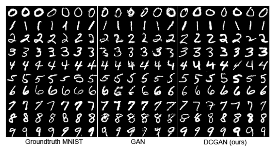
Results

First result compares DCGAN samples with GAN samples, where DCGAN achieves error rate of 2.98% on 50K samples and GAN achieves 6.28% error rate.

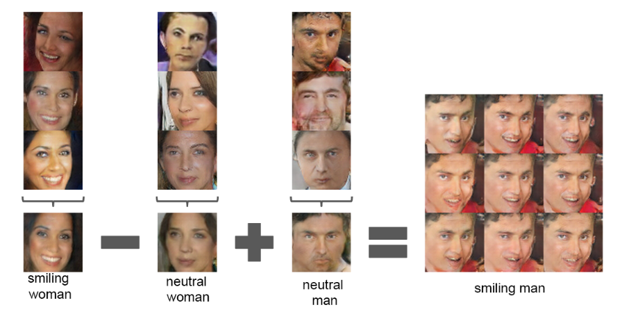
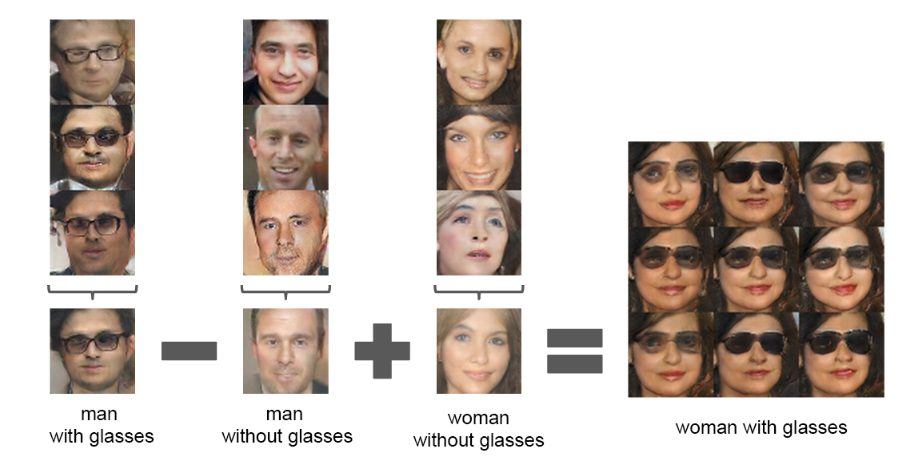
The second most interesting result obtained from paper is, we can perform arithmetic on images to obtain meaningful representation. For e.g. if we take smiling woman subtract neutral woman and add neutral man, we get smiling man as output. Another one is man with glasses - man without glasses + woman without glasses = woman with glasses. Amazing right? Does this remind you of something familiar in case of word vectors, remember?

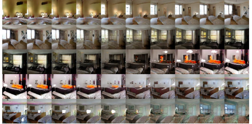
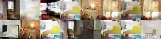
The third result walks through the latent space to see if model has not simply memorized training sample. In first row, we see a room without a window slowly transforming into a room with a giant window and in last row, we see what appears to be a TV slowly being transformed into a window.

WGAN

The generative models makes the model’s distribution close to data distribution either by optimizing distribution using maximum likelihood (Question: Prove that MLE is equal to minimizing KL divergence) or learn a function that transforms existing z (latent variable) into model’s distribution. Authors of the WGAN paper propose a different distance metrics to measure the distance between distributions i.e d(\(p_{data}\), \(p_{model}\)). We have seen that there are many other ways to measure the similarity of two distribution like KL-divergence, Reverse KL-divergence, Jenson-Shannon(JS) divergence for generative model but each of the above methods don’t really converge for some sequence of distribution. (We haven’t provided any formal definition of each of method above and leave it as exercise for readers to explore.) Hence, bring in the Earth Mover(EM) distance or Wasserstein-1. Alex Irpan provides a great overview of WAN’s in general and is great starting point to study WGAN before heading to paper. The intuition behind the EM distance is we want our model’s distribution \(p_{model}\) to move close to \(p_{data}\) true data distribution. Moving mass \(\mathbf{m}\) by distance \(\mathbf{d}\) requires effort \(\mathbf{m}\cdot\mathbf{d}\). The earth mover distance is minimal effort we need to spend to bring these distributions close to each other. Authors provide a proof in paper to why Wasserstein distance is more compelling than other methods and hence a better fit as loss function for generative models. But Wasserstein distance is intractable in practice. So, authors propose alternative approximation which a result from Kantorovich-Rubinstein duality. Sebastion Nowozin provides very excellent introduction to each of the obscure terms above. Finally feast your eyes with WGAN algorithm,

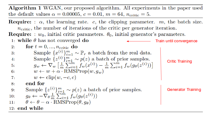
Notice there is no discriminator but a critic and there is something extra term of clipping weights in the algorithm. Also, we train critic for more time \(n_{critic}\) times more than generator. The discriminator in GAN is known as critic in WGAN because the critic here is not classifier of real and fake but is trained on Wasserstein loss to output unbounded real number. \(\mathbf{f_{w}}\) doesn’t give output {0, 1} and that is reason why authors call it critic rather than discriminator. Since the loss for the critic is non-stationary, momentum based methods seemed to perform worse. Hence algorithm uses RMSprop instead of Adam as WGAN training becomes unstable at times when one uses a momentum based optimizer. One of the benefits of WGAN is that it allows us to train the critic till optimality. The better the critic,the higher quality the gradients we use to train the generator. This tells us that we no longer need to balance generator and discriminator’s capacity properly unlike in standard GAN.

In short, take GAN change training procedure a little and replace cost function in GANs with Wasserstein loss function.

After 19 days of proposing WGAN, the authors of paper came up with improved and stable method for training GAN as opposed to WGAN which sometimes yielded poor samples or fail to converge. In this method, authors get rid of use of clipping the weights of critic in WGAN and use a different method which is to penalize the norm of gradient of the critic with respect to its input. This new loss is WGAN-GP.

In short, take GAN change training procedure a little and replace cost function in GANs with WGAN-GP loss function i.e. add gradient penalty term to the previous critic loss.

Results

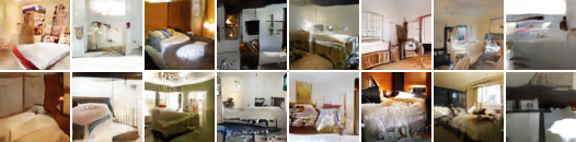
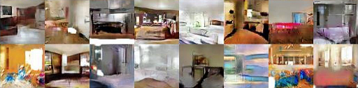
After training on LSUN dataset, here are the results produced. Left from WGAN with DCGAN architecture and right from DCGAN.

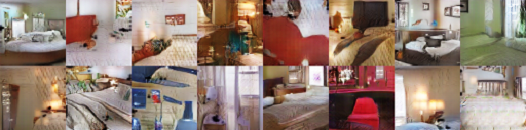
The result below has on left side WGAN with DCGAN architecture and DCGAN on right with both not using batch norm. If we remove batch norm from the generator, WGAN still generates okay samples, but DCGAN fails completely.

Comparing WGAN on left with standard GAN. GAN suffers from mode collapse. This is the phenomenon that after learning for few epochs dataset, the model goes to failure mode and stops learning. The model starts producing same number of images everywhere with very tiny variations.

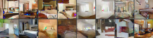
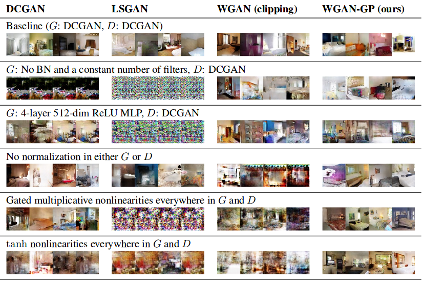
The comparison of results of WGAN with WGAN-GP, DCGAN and LSGAN on LSUN dataset,

Pix2Pix

The researchers at BAIR laboratory devised a method for image to image translation using conditional adversarial networks.The figure below clearly shows what’s going on.

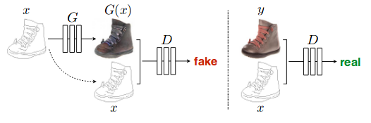
Here Conditional GAN model learns to map edges -> photo. The discriminator D, learn to classify between fake(produced by G) and real {edge, photo} tuples. The generator G learns to fool D. The only difference with previous approach of standard GAN is using conditional GAN. In case of standard GAN, we generator learns mapping from random noise z to output image y, i.e. G : z -> y. In contrast, conditional GANs learns a mapping from observed image x, random noise z to output image y, i.e. G : {x, z} -> y and D : {x, y} will classify if the tuple is real or fake depending on whether y is generated by GAN or is taken from real dataset. Both G and D observe input x. The new loss function to optimize then becomes, \(\mathcal{L}_{cGAN} = \mathbb{E}_{\mathbf{x,y}}[\log_{}(D(x,y)] + \mathbb{E}_{\mathbf{x,z}}[\log_{}(1-D(x, G(\mathbf{x, z})))]\), which is again minmax game G minimizing and D maximizing this objective function.

In short, instead of using standard GAN we use variant called cGAN and accordingly new objective function.

Results

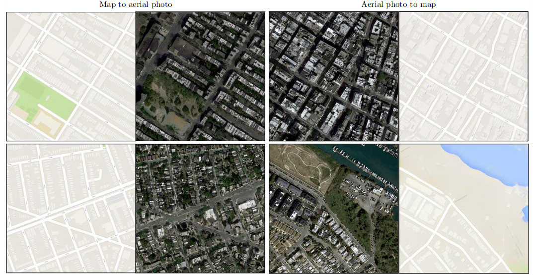
Paper showed some of the fantastic results obtained by using cGANs.

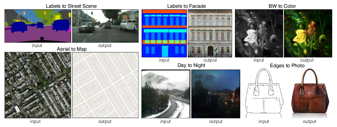
This figure shows how different domains like segmentation, aerial mapping, colorization, etc can be learned using cGANs.

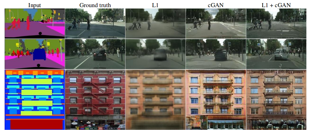
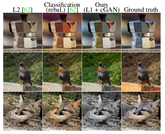
Applying cGANs in domain of semantic segmentation, the result obtained from L1 + cGANs are better than other approaches.

This figure shows input, output i.e. {aerial, map} and {map, aerial} tuples which can both be learned by using cGANs.

This figure shows the result after applying cGAN for colorization along with results from other approaches.

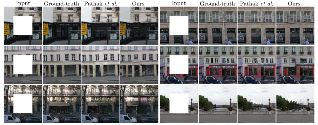
This figure shows uses cGAN for image completion.

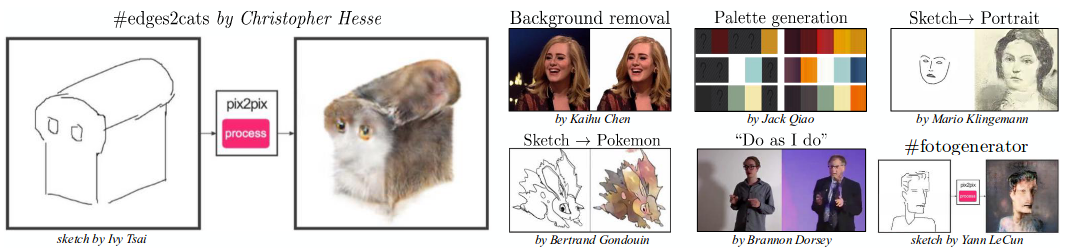
This shows how to convert sketch to image resembling the sketch. Also, use of cGANs to remove background and transferring of pose in “Do as I do” example shown below.

CycleGAN

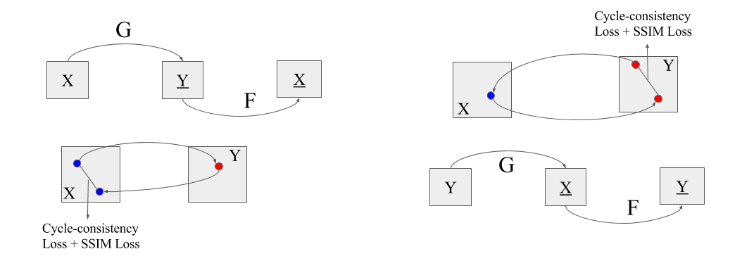
Above we visited pix2pix method where we provided pairs input and output to cGAN to learn mapping. CycleGAN on other hand performs same task in unsupervised fashion without paired examples of transformation from source to target domain. The trick used by CycleGAN that makes them get rid of expensive supervised label in target domain is double mapping i.e. two-step transformation of source domain image - first by trying to map it to target domain and then back to the original image. Hence, we don’t need to explicitly give target domain image. The goal in CycleGAN is to learn the mapping from G : X -> Y such that distribution of images from G(X) is indistinguishable from from the distribution of images of Y. But because this mapping is under-constrained (or not guided), we couple it with an inverse mapping F : Y -> X where we converted the generated image from above mapping back to original image and introduce a cycle consistency loss to enforce F(G(X)) \(\approx\) X and G(F(Y)) \(\approx\) Y. Combining this loss along with individual losses of G and F, we get the full objective for unpaired image-to-image translation. This is so good that we will repeat again with the figure below.

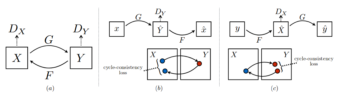
There are two generators(mapping functions) G : X -> Y and F : Y -> X, and two discriminators \(D_{X}\) which aims to distinguish images of X(real) & F(Y)(fake) samples and \(D_{Y}\) which aims to distinguish images of Y(real) & G(X)(fake) samples. \(D_{Y}\) encourages G to translate X into outputs indistinguishable to Y, and similarly \(D_{X}\) encourages F to translate Y into outputs indistinguishable to X. The (b) and (c) part are forward and backward cycle-consistency loss introduced to capture the intuition that if we translate from one domain to the other and back again we should arrive at where we started. Forward cycle-consistency in (b) is x -> G(x) -> F(G(x)) \(\approx\) x and backward cycle-consistency in (c) is y -> F(y) -> G(F(y)) \(\approx\) y. If we want to write the total loss mathematically,

\[\begin{aligned} \mathcal{L}_{GAN}(G, D_{Y}, X, Y) &= \mathbb{E}_{\mathbf{y} \sim p_{data}(y)}[\log_{}(D_{Y}(y)] + \mathbb{E}_{\mathbf{x} \sim p_{data}(x)}[\log_{}(1 - D_{Y}(G(x)))] \\ \mathcal{L}_{GAN}(F, D_{X}, Y, X) &= \mathbb{E}_{\mathbf{x} \sim p_{data}(x)}[\log_{}(D_{X}(x)] + \mathbb{E}_{\mathbf{y} \sim p_{data}(y)}[\log_{}(1 - D_{X}(F(y)))] \\ \mathcal{L}_{cyc}(G, F) &= \mathbb{E}_{\mathbf{x} \sim p_{data}(x)} ||F(G(x)) - x|| + \mathbb{E}_{\mathbf{y} \sim p_{data}(y)} ||G(F(y)) - y|| \\ \mathcal{L}(G, F, D_{X}, D_{Y}) &= \mathcal{L}_{GAN}(G, D_{Y}, X, Y) + \mathcal{L}_{GAN}(F, D_{X}, Y, X) + \lambda\mathcal{L}_{cyc}(G, F) \end{aligned}\]

In short, cycle GAN is unsupervised learning variant of standard GAN where we learn to translate images from source to target domain.

Results

This paper produced most amazing results. Just keep watching.

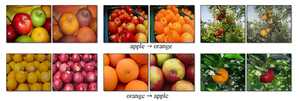
Horse -> Zebra, really?

Image-to-image translation can be done in many ways. For example, turning winter images to summer and vice versa, turning horses to zebras and vice versa, turning any photo into Monet style and vice versa.

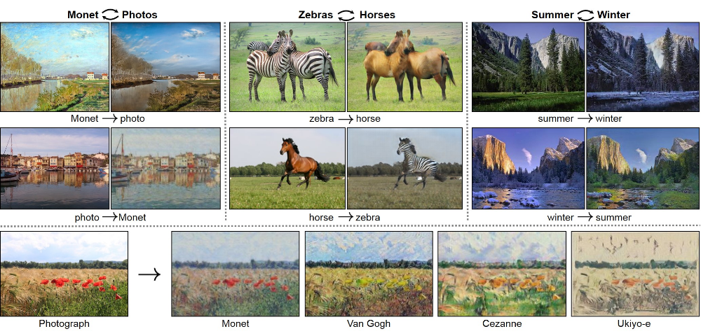
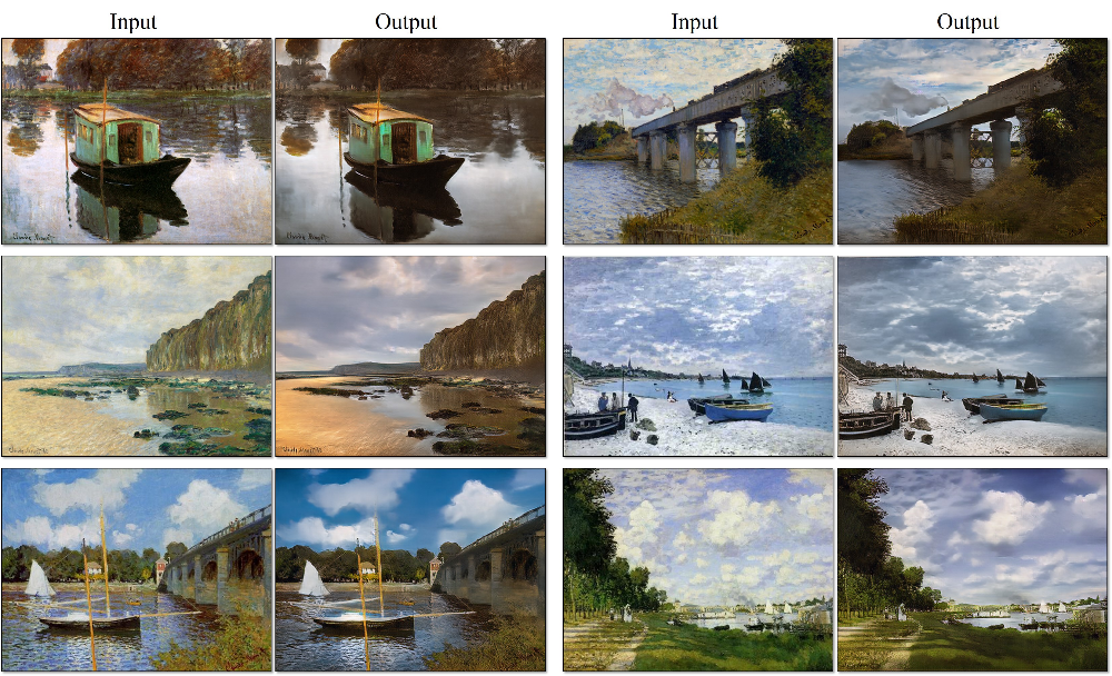
Here is result of mapping Monet style paintings into photos.

Here is the opposite result of turning photos into different styles of painting like Monet, Van Gogh, etc. Do they look familiar to something we did previously? Yes, Neural Style Transfer.

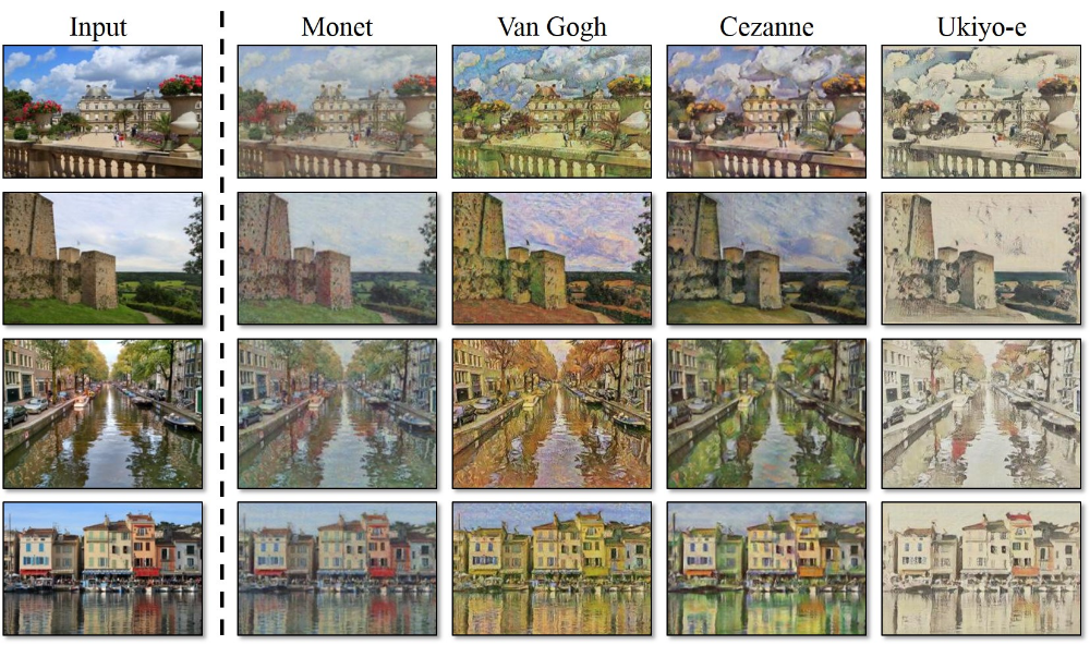
Who says we need apple to apple comparison?

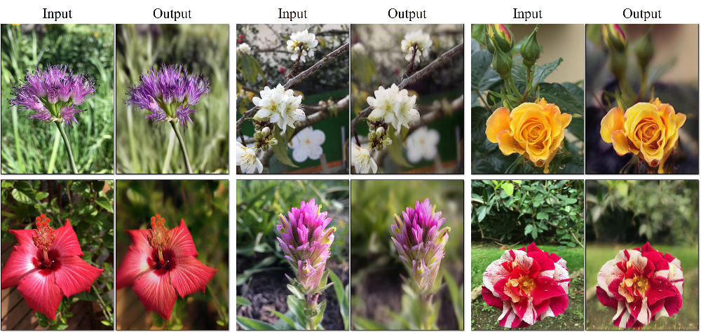
This result shows photo enhancement achieved by mapping snaps from smartphone to the ones taken on DSLR.

ProGAN

Generating images from 32x32 upto 128x128 with all the new fancy losses seemed cool but generating images of large resolution say 512x512 remained a challenge. The problem with large resolution is that large size implies small minibatches which in turn lead to training instability. We have already visited how training GANs can lead to mode collapse where every output of GAN is some fixed number of same images where discriminator wins and generator loses and it’s game over. These all problems are the reason why GANs cannot achieve high quality even if we try to make GANs deeper or bigger.

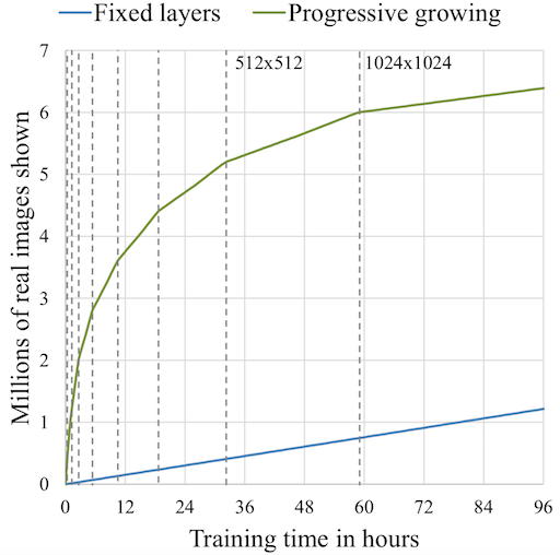
The team at Nvidia tackled this challenge through new GANs called ProGAN and bunch of other tricks. The idea behind ProGAN is we start with low resolution images, and then progressively increase the resolution by adding layers to the networks. What happens is instead of using standard GANs where we would have used deep networks to generate high res from latent code, and as the networks are deep it would have taken a lot of time for G to come up with good high res images as D will be already better in rejecting in these samples. This increase in amount of time can lead to mode collapse as already D is better at what it is doing and G is failing to learn anything as layers are deeper and going from randomly initialized weights of each layer to good weight will take a lot of time, if at all possible. So, instead of using standard GANs, the team at Nvidia came up with something called ProGAN. ProGAN starts with tiny images of size 4x4 images and correspondingly shallow networks. The network is trained with this size for sometime until they are more or less converged which will be lot less as network is small, next shallow network corresponding to size 8x8 is added which is again trained till convergence and further 16x16 image size network is added. This continues till sizes up to image resolution of 1024x1024 and after 2 days of training these ProGANs we get amazing results. How would G and D look? They would be mirror of each other. In case of 4x4, G will take latent code and produce 4x4 images and D will take 4x4 and produce real output number(unbounded), as authors use WGAN-GP as loss instead of real and fake. Let’s see how it looks,

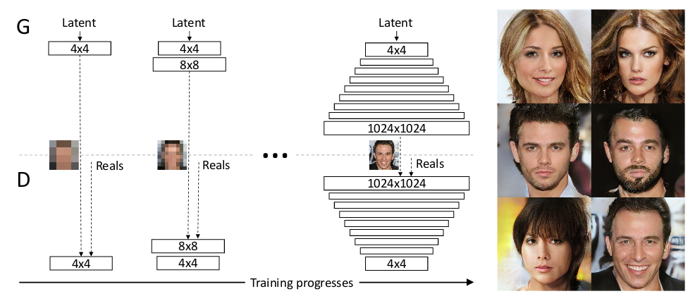
This is how typical training in ProGAN looks like.

ProGAN generally trained about 2–6 times faster than a corresponding traditional GAN depending on the output resolution.

Here is a typical architecture of ProGAN shown below. The generator architecture for k resolution follows same pattern where each set of layers doubles the representation size and halves the number of channels and discriminator doing the exact opposite. The ProGAN uses nearest neighbors for upscaling and average pooling for downscaling whereas DCGAN uses transposed convolution to change the representation size.

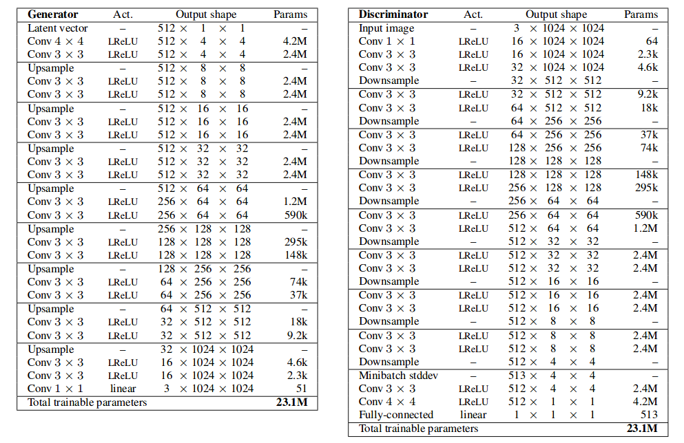
That’s a very high level overview, but let’s dwell on this a bit because they are so cool! Let’s look at one such architecture of ProGAN.

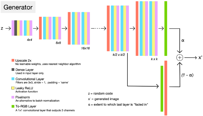
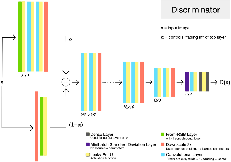
Look at the architecture G and D on left side we see that they are exact mirrors of each other. Let’s walk through up to some kxk resolution and see what happens in detail. First generator starts with producing 4x4 image resolution and passing it to D and all backpropagation of error and learning of G and D takes place until some degree of convergence. So we trained for only 3 layers in G and 3 layers in D for 4x4 resolution which takes a lot less time. Next, to generate double the resolution 8x8 image, we add 3 more layer to each side of G and D. Now, all the layers in G and D are trainable. To prevent shocks in the pre-existing lower layers from the sudden addition of a new top layer, the top layer is linearly “faded in”. This fading in is controlled by a parameter \(\alpha\), which is linearly interpolated from 0 to 1 over the course of many training iterations. So, there is no problem of catastrophic forgetting and only new layers are learned from scratch. This reduces the training time. Next time when we add 3 more layers to increase the resolution of size to 16x16, they are faded-in with already present 4x4 and 8x8 blocks and this ways G and D fight each other using WGAN-GP as loss function up to a desired number of resolution.

To further increase the quality of images and variation, authors propose 3 tricks such as pixel normalization(different from batch or layer or adaptive instance normalization), minibatch standard deviation and equalized learning rate. In minibatch standard deviation, D is given a superpower to penalize G if the variation between training images and the once produced by G is high. G will be forced to produce same variation as in training data. To achieve this equalized learning rate, they scale the weights of a layer according to how many weights that layer has using. This makes sure all the layers are updated at same speed to ensure fair competition between G and D. Pixelwise feature normalization prevents training from spiraling out of control and discourages G from generating broken images.

And the last contribution made was how to evaluate two G’s, which one is better? This can be done through Sliced Wasserstein Distance (SWD) where we generate large number of images and extract random 7x7 pixels neighborhood. We interpret these neighborhood points as in 7x7x3 dimensional space and comparing this point cloud against the real images(same process) point cloud which can be repeated for each scale.

In short, using ProGAN we can generate high res images.

Results

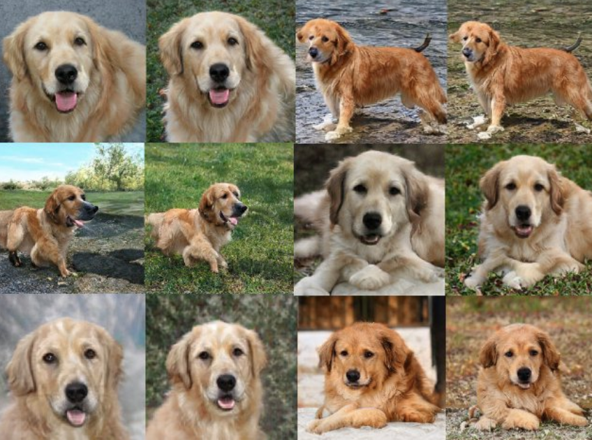
I will let the results speak for themselves. Remember none of these faces are real or from training dataset. They are synthesized by G totally from scratch.

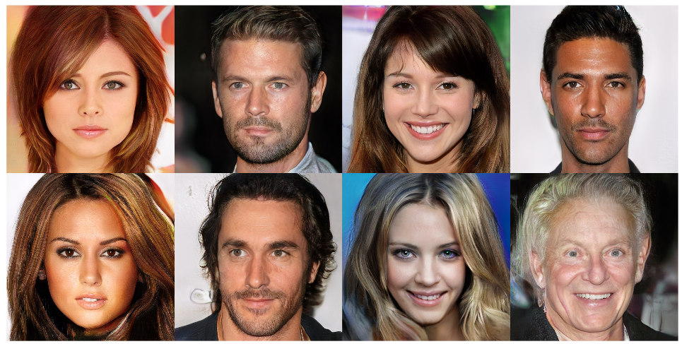
After walking the latent space which is continuous, one such output is this. Notice the changes to hairs, expression, shape of face. Amazing!

StyleGAN

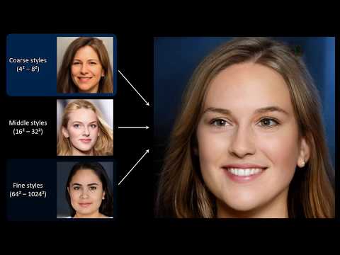
ProGAN was pretty mouthful, right? The authors of Nvidia came out with this paper called StyleGAN where we can by modifying the input of each level separately, control the visual features that are expressed in that level, from coarse features (pose, face shape) to fine details (hair color), without affecting other levels. What this means? Let’s look at example below and understand what this means.

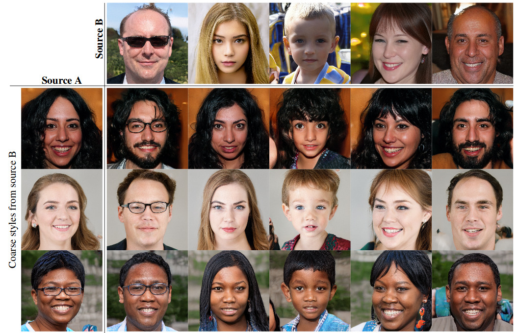
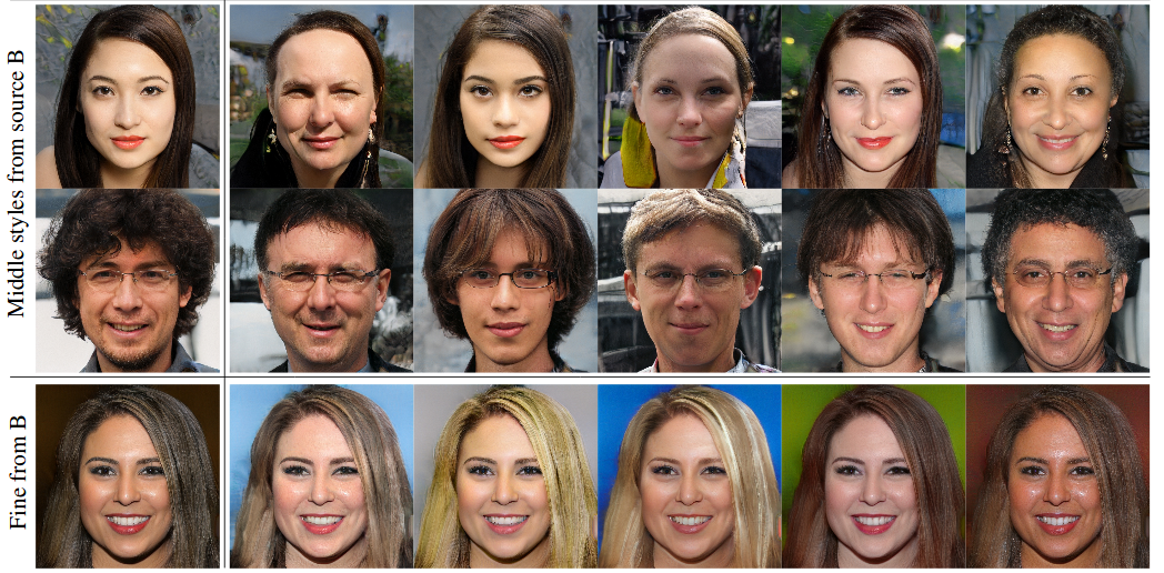
We are copying the styles from different resolutions of source B to the images from source A. Copying the styles corresponding to coarse spatial resolutions (\(4^{2}\)–\(8^{2}\)) brings high-level aspects such as pose, general hair style, face shape, and eyeglasses from source B, while all colors(eyes, hair, lighting) and finer facial features resemble A. If we instead copy the styles of middle resolutions (\(16^{2}\)–\(32^{2}\)) from B, we inherit smaller scale facial features, hair style, eyes open/closed from B, while the pose, general face shape, and eyeglasses from A are preserved. Finally, copying the fine styles (\(64^{2}\)–\(1024^{2}\)) from B brings mainly the color scheme and microstructure.

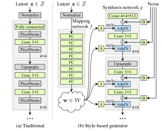
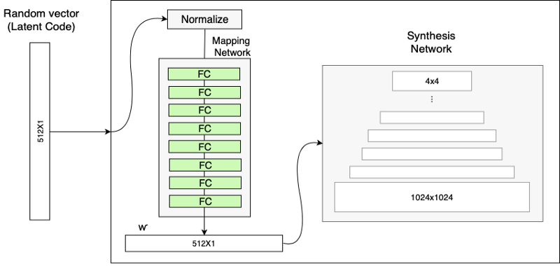
How does it work then? StyleGANs are upgraded version of ProGAN where we can each progressive layers can be utilized to control different visual features of image. The generator in StyleGAN starts from a learned constant input and adjusts the “style” of the image at each convolution layer based on the latent code, therefore directly controlling the strength of image features at different scales. As we saw from above example, coarse styles can be controlled using \(4^{2}\)–\(8^{2}\) resolution, middle styles controlled by \(16^{2}\)–\(32^{2}\) resolution layers and finer styles using \(64^{2}\)–\(1024^{2}\) resolutions. The typical ProGAN shown on the left side in image above uses progressive layer training to produce high resolution images but StyleGAN uses a different generator approach. Instead of mapping latent code z to resolution, it uses Mapping Network, which maps the latent code z to an intermediate vector w. The latent vector is sort of like a style specification for the image. The purpose of using different mapping network is suppose we wanted change the hair color of image by nudging the value in latent vector, but what if output produces different gender, or glasses, etc. This is called feature entanglement. The authors state that the intermediate latent space is free from that restriction and is therefore allowed to be disentangled. The mapping network in the paper shown in images above consists of 8 fully-connected layer and produce w of size 512x1.

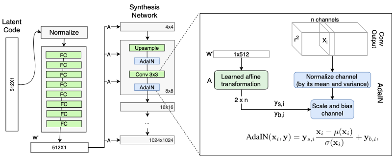
We can view the mapping network and affine transformations as a way to draw samples for each style from a learned distribution, and the synthesis network as a way to generate a novel image based on a collection of styles. This synthesis network takes in the output generated by mapping network to generate image by using AdaIN with whom we had encounter with before here. Synthesis network allows us to make small changes to the input latent vector without making the output image/face look drastically different. The input to synthesis network is a constant values of size 4x4x512. The authors found that the image features are controlled by w and the AdaIN, and therefore the initial input can be omitted and replaced by constant values.

There are other tricks such as style mixing which is used as regularization to reduce the correlation between the level in synthesis network. Interesting thing which we can perform with style mixing is to see what happens when we combine two images. The model combines two images A and B generated by taking low level-features from A and high-level features from B. Another trick used in paper is truncation trick in W. The authors use a different sampling method such as truncated or shrunk sampling to sample latent vectors.

In short, this paper using StyleGANs details not only how to generate high quality images but how to control different styles of the generated image making them more unbelievable fake images.

Results

Video contains a lot many examples of style mixing, interpolation and various ablation studies of different parameters.

BigGAN

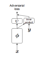
The team at Deepmind showed that GANs benefits from scaling and trained models with two to four times as many parameters and eight times the batch size compared to prior art. BigGANs uses class-conditional GANs where they pass class-information to G and to D using projection as shown in image below on left side, where they pass class information using inner-product with output of D. The objective used by BigGAN is hinge loss. BigGAN adds direct skip-connections from noise vector z to multiple layers of G rather than just initial layer in standard GANs. The intuition behind this design is to allow G to use the latent space to directly influence features at different resolutions and levels of hierarchy. The latent vector z is concatenated with class embeddings and passed to each residual block through skip connections. Skip-z provides a modest performance improvement of around 4%, and improves training speed by 18%. Residual Up used for upsampling in BigGAN G’s shown in (b) and Residual Down for downsampling in BigGAN D’s is shown in (c).

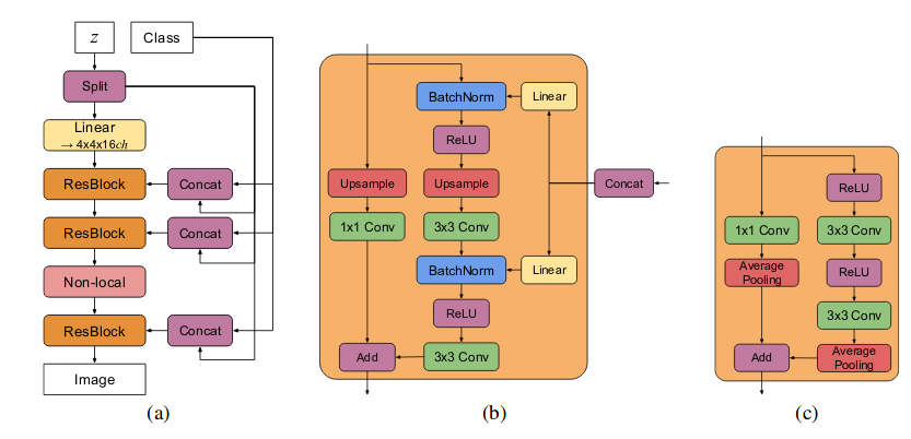
BigGAN also employed few tricks such as Truncation Trick, where in previous literature of GAN latent vectors z are drawn from either \(\mathcal{N}\)(0, 1) or \(\mathcal{U}\)[-1, 1]. Instead BigGAN latent vectors are sampled from truncated normal distribution where values which fall outside a range are resampled to fall inside that range. Authors observe that using this sampling strategy does not work well with large models and hence add a Orthogonal Regularization as penalty. One important conclusion drawn from this is that we do not need to use explicit multiscale method as used in ProGAN and StyleGAN for producing higher resolution images. Despite these improvements, BigGAN undergoes training collapse. The authors explore in great-detail why it happens so through colorful plots. They also provide results and conclusion of large amount of experiments performed from which a lot can be learned.

In short, BigGAN could do what ProGAN thought would require multi-scale approach in single-scale by using some tricks.

Results

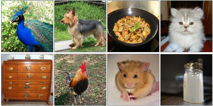
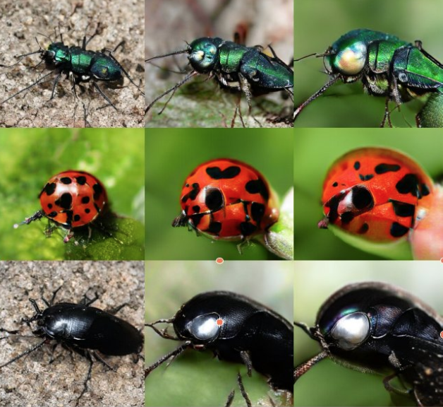
Jaw-dropping moment 🤪. All the images generated by generator from scratch. Get outta here!

Zaid Alyafeai provides different tricks we can perform in latent space.

Breeding : In this we breed between two different classes, i.e we create intermediate classes using a combination of two different classes.

Background Hallucination : Here we try to change the background keeping the foreground object the same.

Natural Zoom : We zoom into certain generated image to look into finer details. It’s amazing.

Here is example of walking in latent space for specific z and c pairs,

GAN semi-supervised learning

In paper Improving GAN by training, authors demonstrate they are able to achieve 99.14% accuracy with only 10 labeled examples per class with a fully connected neural network on MNIST dataset. The basic idea of semi-supervised learning with GANs is to use feature matching objective and add extra task for discriminator i.e. in addition to classify it will also predict the label of the image. The fake samples of generator can be used as dataset for which discriminator will predict a class corresponding to that image. The feature matching objective is a new objective for G, to train the generator to match the expected value of the features on an intermediate layer of the discriminator. If \(f(\mathbf{x})\) denote activations on an intermediate layer of the discriminator, then new objective for generator is defined as \(\Vert\mathbb{E}_{\mathbf{x} \sim p_{data}(\mathbf{x})}[f(\mathbf{x})] - \mathbb{E}_{\mathbf{z} \sim p_{z}(\mathbf{z})}[f(G(\mathbf{z}))]\Vert^{2}_{2}\). Feature matching is effective in situations where regular GAN becomes unstable.

Speech

Okay, enough about images. Show me(GAN) what else you got. Synthesizing speech is one the cool areas where GANs have played a significant role. And with good comes bad, “deepfake” voice technology.

GANSynth

Magenta has a great blog with example outputs of audio generated, definitely worth a look! To be frank, I didn’t get a lot out of paper. Previous approach for speech synthesis was using Autoregressive models – another type of generative model – like WaveNet, which have slow iterative sampling and lack global structure(no idea what this means). They make use of ProGAN(which we looked above) to generate audio spectra. Briefly, model samples a random vector z from from a spherical Gaussian and runs it through a stack of transposed convolutions to upsample and generate output data, x = G(z). This generated output is fed into discriminator D of downsampling convolutions (whose architecture mirrors the generator’s) to estimate a divergence measure between the real and generated distribution. WGAN-GP is used as objective function same as used in ProGAN. Rather than generate audio sequentially as done in WaveNet, GANSynth generates an entire sequence in parallel, synthesizing audio significantly faster than real-time on a modern GPU and ~50,000 times faster than a standard WaveNet.

In short, it works. GANs synthesize musics. Mozart we(Magenta) are coming for you!

Results

A lot many audio samples generated by GANSynth and it’s comparison with real audio samples can be found on the blog.

Text

What else you got? We have seen a lot of NLP but now the question is are GANs good enough to fool the discriminator oops the world? We will look into one such study by introducing an actor-critic conditional GAN that fills in missing text conditioned on the surrounding context, aka MaskGAN.

MaskGAN

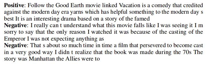
We have seen previously how RNN and seq2seq language models are conditioned on previous words to generated words sequentially. This makes them difficult to generate samples that were not present in the training. The paper uses GAN along with REINFORCE algorithm (belonging to family of policy gradient) from reinforcement learning (which we will study soon 🙌). So for now we take author’s word that it works and according to human evaluations, MaskGAN generates significantly better samples that maximum likelihood trained model.

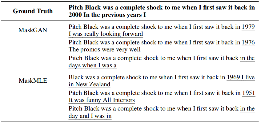
Results

Here are some of the results produced by MaskGAN along with MaskMLE.

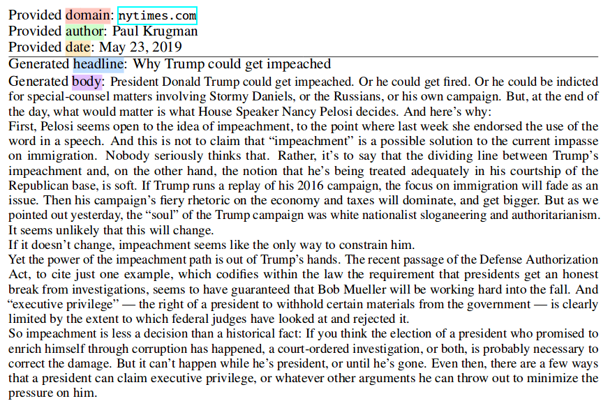
MaskGANs move aside and make some space for GPT-2. We have already dissected this model. We saw what the model was capable of and the aftermath effects are still being echoed everywhere. A very recent paper from Allen Institute for Artificial Intelligence presents GROVER to detect fake news. In this paper, authors propose an adversarial game to detect fake news. There is an “Adversary” whose goal is to generate fake stories that match specified attributes: generally, being viral or persuasive. The stories must read realistically to both human users as well as the verifier. And then there is “Verifier” whose goal is to classify news stories as real or fake. The verifier has access to unlimited real news stories, but few fake news stories from a specific adversary. Remember how G and D were fitting to be good, the same case will be observed here. Adversary will produce good fake stories and Verifier will get good at classifying stories real or fake.

And now bringing you the fake articles generated by Adversary. Real?

Everybody’s favourite startup “Uber for Dogs”.

A similar tool called Catching a Unicorn with GLTR, to detect automatically generated text from a collaboration of MIT-IBM Watson AI lab and HarvardNLP group. Check out Live Demo

Videos

GANs for video has mind blowing applications. Remember deepfakes, the one which everyone is worried about. Yes, it was born here. The literature for GANs in video is large, we will particularly sample 2 applications, deepfakes and everybody can dance.

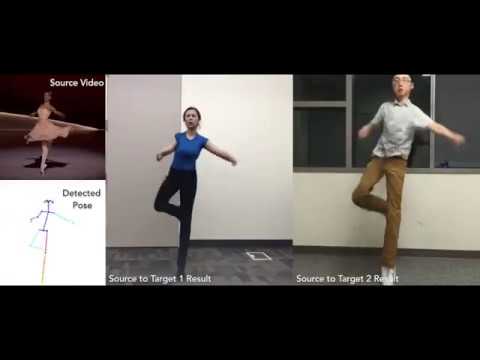
Everybody can dance

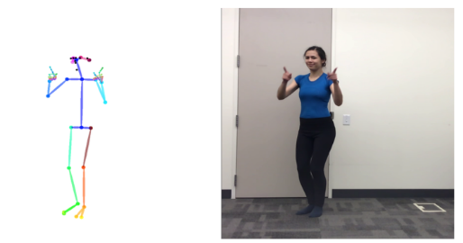
Can you dance? Don’t worry if you can’t. We will let GANs teach us alright ready? The researchers at Berkeley presented a simple method for “do as I do” motion transfer : given a source video of a person dancing we can transfer that performance to a novel (amateur) target after only a few minutes of the target subject performing standard moves. Cool right??? How can be pose this problem looking that above approaches in GAN images? Yes, image-to-image translation between source and target sets. But we do not have corresponding pairs of images of the two subjects performing the same motion to perform supervise translation directly. In pix2pix method, we had {edge, photo} as tuple where edge is passed to both G and D and G generates a fake photo and passes to D to fool it. Even if both subjects were performing same motion, it would difficult to have exact frame body-pose correspondence between source to target due to body shape and stylistic differences unique to each subject. How can we proceed further? Keypoint-based pose. Keypoints encode body position irrespective of shape and styles, hence keypoint can act as our intermediate representation between two subjects. Obtaining pose for each frame from target video we get pairs of (pose stick figure, target person image). Here is one such example,

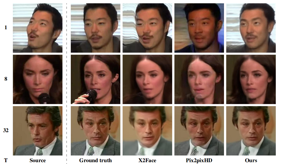
As trained in pix2pix, we can train a image-to-image translation model between pose stick figures and target person image. To transfer the motion of source to target, we input pose stick figure of source and output the same pose for specific target subject as a image. To encourage the temporal smoothness of generated videos, the authors condition the prediction at each frame on that of the previous time step. To increase facial realism in their results they include a specialized GAN trained to generate the target person‘s face. Let’s take a close look at the training and inference pipeline.

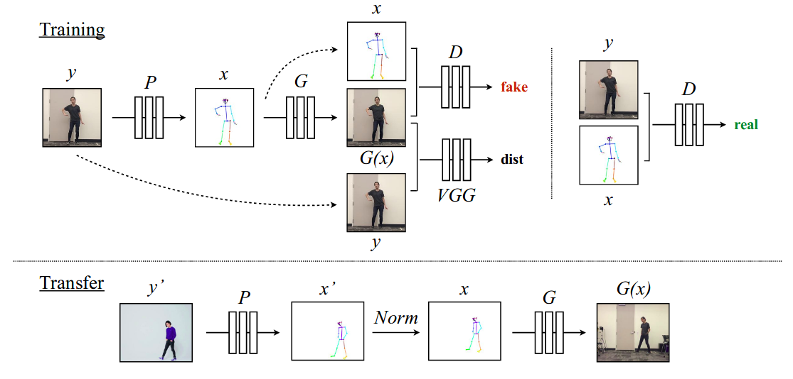
First training pipeline, for a given frame \(\mathbf{y}\) from target video, it passed through pose detector P to obtain a corresponding target pose stick figure, \(\mathbf{x} = P(\mathbf{y})\). We have pairs of (\(\mathbf{x}\), \(\mathbf{y}\)) which we can pass through G which learns the mapping and synthesizes target image pairs given pose stick figure. Now, the generated image G(\(\mathbf{x}\)) is passed along with pose stick figure to D, where D learns to distinguish the real and fake pairs i.e. “real pairs” (pose stick figure \(\mathbf{x}\), ground truth target image \(\mathbf{y}\)) and “fake pairs” (pose stick figure \(\mathbf{x}\), generated target image G(\(\mathbf{x}\))). This training is done end-to-end with adversarial loss with objective function similar to that in pix2pixHD and perceptual reconstruction loss (dist) from VGGNet to make G(\(\mathbf{x}\))) resemble more like ground truth image (\(\mathbf{y}\)).

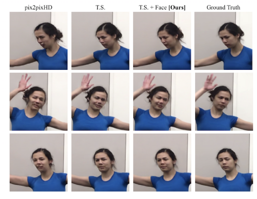
Next transfer pipeline, similar to training pose detector P extracts pose information from source video frame \(\mathbf{y}^{'}\) yielding pose stick figure \(\mathbf{x}^{'}\). However, in their video the source subject likely appears bigger, or smaller, and standing in a different position than the subject in the target video. In order for the source pose to better align with the filming setup of the target, we apply a global pose normalization Norm to transform the source’s original pose \(\mathbf{x}^{'}\) to be more consistent with the poses in the target video \(\mathbf{x}\). Then we pass the normalized pose stick figure \(\mathbf{x}\) into our trained model G to obtain an image G(\(\mathbf{x}\)) of our target person which corresponds with the original image of the source \(\mathbf{y}\). To further improve the quality of video, authors use GANs for temporal coherence and adding more detail and realism to face. Here is comparison of different results, such as use only pix2pixHD objective, temporal smoothing and finally both TS & face approach as described in paper as compared to ground truth. Clearly, using TS and Face GAN we obtain better results.

Results

This video is sufficient enough to convey the awesomeness achieved.

Deepfakes

Deepfakes created a lot of buzz and I mean a lot, lot and there is a YouTube channel for it too. We will be looking at two types of deepfakes : the face-swapping one and mona-lisa speaking one. We will explore both.

Faceswap GAN

Let’s start with face-swapping GANs. Many of you can guess what GANs will be particularly helpful here. Did I hear CycleGAN? Yes, absolutely correct. All we need to do is unsupervised training to two sequences of unaligned video frames from each person. But authors of the paper suggested some improvements to CycleGAN that deals with the common problem of mode collapse, to capture details in facial expressions and head poses, and thus transfer facial expressions with higher consistency and stability. The loss function used in CycleGAN, \(\mathcal{L}(G, F, D_{X}, D_{Y}) = \mathcal{L}_{GAN}(G, D_{Y}, X, Y) + \mathcal{L}_{GAN}(F, D_{X}, Y, X) + \lambda\mathcal{L}_{cyc}(G, F)\) proved to be challenging to get good transferring results on unaligned datasets. So in order to generate better face-off sequences on unaligned datasets instead authors proposed adding two losses, WGAN loss to prevent mode collapse in adversarial training and to achieve more stable results. SSIM Loss (Structural Similarity) matches the luminance(l), contrast(c), and structure(s) information of the generated image and the input image, and it’s proved to be very helpful to improve the quality of image generation. Here is how the architecture looks with new added loss of WGAN, SSIM in addition to cyclic consistency loss(\(L_{cyc}\)).

While transferring face one thing to be noted is how we will deal with foreground and background i.e. the background of the source video should remain the same only the face of the subject from the source video should be swapped with that of target subject. So, authors propose a trick to segment the input faces and then fed the mask as weight on pixel-reconstruction error. Generator uses variant of U-Net architecture and discriminator 5-layer Conv and also experimented with using two discriminator whose losses will be averaged given some weight \(\lambda\) in final loss function. The results obtained from the experiments were noisy, don’t deal with scale, very shaky and inconsistent between the frames.

Results

How about we settle for video as a result? This result is not obtained from the model trained on above paper. But it surely uses CycleGAN just with some modifications (which I don’t know what, will have to ask author?).

Mona Lisa speaking GAN

We have seen how brilliant GANs are spitting out beautiful and realistic looking image. The team of researchers at Samsung AI published a paper where they create a personalized talking head model with only few-images. The few-shot learning ability is obtained through extensive pretraining (meta-learning) on a large corpus of talking head videos corresponding to different speakers with diverse appearance. In the course of meta-learning , system simulates few-shot learning tasks and learns to transform landmark positions into realistically-looking personalized photographs, given a small training set of images with this person. After that, a handful of photographs of a new person sets up a new adversarial learning problem with high-capacity generator and discriminator pretrained via meta-learning. The new adversarial problem converges to the state that generates realistic and personalized images after a few training steps. If nothing made sense so far, no worries we will break down everything. Starting from architecture,

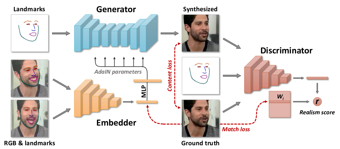
There will be two pipelines, training and fine-tuning for inference. First training, also meta-learning stage assumes that we have M video sequences, containing talking heads of different people. We denote \(\mathbf{x_{i}}\) the i-th video sequence and with \(\mathbf{x_{i}(t)}\) it’s t-th frame. All the training happens in episodes of K-shot learning (K=8). In each episode, we randomly draw a training video sequence i and a single frame t from that sequence. In addition to t, we randomly sample additional K such frames \(s_{1},...s_{K}\) from the same sequence. Let’s consider one frame \(\mathbf{x_{i}(t)}\) which is passed through landmark detection algorithm to get resultant landmark image \(\mathbf{y_{i}(t)}\). Then embedder E(\(\mathbf{x_{i}(s)}\), \(\mathbf{y_{i}(s)}\), \(\phi\)) takes video frame and produces a output N-dimensional vector \(\mathbf{\hat{e}_{i}(s)}\). The \(\phi\) are networks learning parameters and \(\mathbf{\hat{e}_{i}(s)}\) contains video-specific information such as person’s identity independent of pose. \(\mathbf{\hat{e}_{i}}\) is sent to generator G(\(\mathbf{y_{i}(t)}\), \(\mathbf{\hat{e}_{i}}\) ; \(\psi\), P) takes in input landmark information of video frame i.e. \(\mathbf{y_{i}(t)}\) not seen by embedder, predicted video embedding \(\mathbf{\hat{e}_{i}}\) and produces output \(\mathbf{\hat{x}_{t}}\). There is one catch in G, all the parameters in G are split into 2 groups: the person-generic parameters \(\psi\), and the person-specific parameters \(\hat{\psi}_{i}\). During meta-learning only \(\psi\) is trained and \(\hat{\psi}_{i}\) are predicted from \(\mathbf{\hat{e}_{i}}\) and P : \(\hat{\psi}_{i}\)=P\(\mathbf{\hat{e}_{i}}\). We will shortly see why. The discriminator D(\(\mathbf{x_{i}(t)}\), \(\mathbf{y_{i}(t)}\), i) now plays the same role it played in pix2pix or bigGAN i.e. conditional projector discriminator takes input the frame, landmarks corresponding to that frame and learns to distinguish if they are real or fake. The input frame can be real or generated by G. G learns to maximize the similarity of generated image and real frame. Discriminator D learns to distinguish real pair and fake pair. Here a pair consists of landmark image of the frame and ground truth image of that frame or generated output corresponding to that landmark image. The loss function contains 3 parts : (i) Content loss term, which measures the distance between ground truth image \(\mathbf{x_{i}(t)}\) and reconstruction by G \(\mathbf{\hat{x}_{t}}\) using specific layer from VGG16 and VGGFace, L1-loss is combined together with predefined given weight. (ii) The usual adversarial loss term, in addition to realism score which is the output of D contains a additional term of feature matching. This term is introduced to ensure perceptual similarity and also helps in stabilizing the training. (iii) The projection discriminator contains matrix W whose columns correspond to the embeddings to the individual videos. But we already have embedding vector \(\mathbf{\hat{e}_{i}}\) which also contains embeddings of the video, so what the last term in loss does is encourage the similarity of the two embeddings. In addition to above losses, discriminator is updated by minimization of hinge loss. That completes the training pipeline.

Next, once the meta-learning is converged we can leverage this to synthesize talking head sequences for a new person, unseen during meta-learning stage. This is what is covered in fine-tuning step using few-shots. We will use the embedder E from above trained model to calculate embedding vector for some predefined T frames of unseen video. Now G will take the new E embedding vector to generate the image of unseen person but there appears to be some identity gap(person appears to be different than video) so to resolve that we fine-tune using some frame of that video. The generator G now uses \(\hat{\psi}\) which is person-specific parameter along with \(\psi\). This new output frame when trained resembles more like that of person in unseen video. There are some tricks which are done while initializing the weight of D, and D as before outputs a realism score. The new objective contains first two terms from above loss function and also the hinge loss of D.

All of this is simplified a bit but paper details all the necessary steps and different ablation studies with respect to losses.

In short, using meta-learning we send the K-frames to embedding network which send output information about person in video irrespective of person’s pose. Given landmarks and pose independent vector, G learns to map these input to generate a image that looks similar to that of person in video for given landmark. Now, D which is a conditional projector discriminator(same as seen in BigGAN) takes these as inputs and learns to distinguish if the pairs are real or fake. The training objective contains 3 loss terms. When we want to output for new unseen video, we finetune the unseen video for some T frames by modifying G and D a bit and training with new loss function.

Results

Speaking Mona Lisa how about that?

This is the output of fewshot learning for T frames on video of person not seen in meta-learning stage compared to different GANs.

Problems in GANs

As always in an another fantastic blog on distill.pub, the authors of the blog discusses some of the open questions in the field of GANs and about what we know about GANs. Here are the questions :

Will GANs Rule the World?

GANs are getting better and better as if they are on steroids. Does this mean we are doomed? Will GANs rule the world? We are seeing all these cool results with images and videos, the one with the deepfakes, fake speech, etc. This does have serious implications on the society. Are there any counter measures we should be aware of? Sherlock would say, “Don’t worry my dear Watson, if you possess Art of Observation.”

Images

The progress of image generating quality of GANs is shown below.

In an excellent blog by Kyle McDonald helps us to observe. I will mention 2-3 observations. In addition to test your skills you can play this game.

Asymmetry

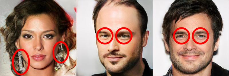
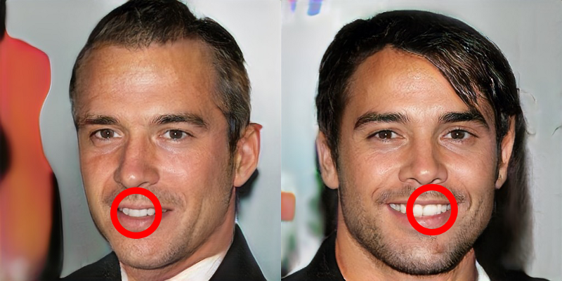
Weird Teeth

Missing Earing

Also, researchers at University of Washington in their Calling Bullshit project have complied some more list of such observations.

Speech

What do you think about this? GANs can be also used to impersonate someone. Don’t believe me, read it here. Using this approach it is possible to assume any age, gender, or tone you’d like, all in real time. Or to take on the voice of a celebrity. Now how about that? In an another interesting researched not related to GAN dubbed as “Speech2Face”, MIT researchers trained a machine learning model to reconstruct a very rough likeness of someone’s face based only on a short audio clip. The cool thing about paper is that they bring into light some ethical consideration posed by this research such as Privacy and Dataset bias.

Videos

Videos particularly deepfakes well know for their realistic impersonation of any person generated by deep learning algorithms such as GANs or other algorithms have surely been a very much topic of interest. Even the former POTUS was surprised with the fake sync lip that circulated Internet last year and expressed concern against such technologies. One can only imagine what devious ways we can use it for and potentially amplify it using social media. The threats of deepfakes may seem innocuous for now but what happens if we when one day when we cannot distinguish what is fake or what is real? What if G become so good that we as D become fooled by generated samples?

Let’s not paint a picture that GANs are bad, I mean they are most interesting idea in last 10 years but there is always a bad side for good side. Moving forward, let’s work put some counter measures and learn from past mistakes so as to not repeat the same history all over again. “With great innovation, comes a great responsibility.”

Special Mentions

Lastly, we apologize to the rest of the GAN family for not mentioning them. But here are some results of special mentions worth showing.

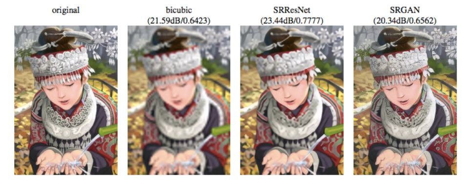
SRGAN : SRGAN paper demonstrates excellent single-image super resolution results that show the benefit of using a generative model trained to generate realistic samples.

iGAN: A user can draw a rough sketch of an image,and iGAN uses a GAN to produce the most similar realistic image. Here is a video demonstration of iGAN,

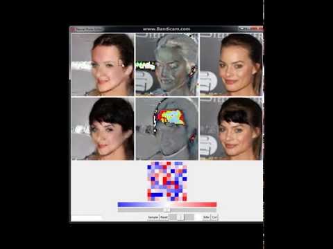
IAN: Using IAN, the user paints rough modifications to a photo, such as painting with black paint in an area where the user would like to add black hair, and IAN turns these rough paint strokes into photo realistic imagery matching the user’s desires. Here is one such demonstration,

GAN Dissection : GAN Dissection is a visualization tool that helps researchers and practitioners better understand their GAN models.

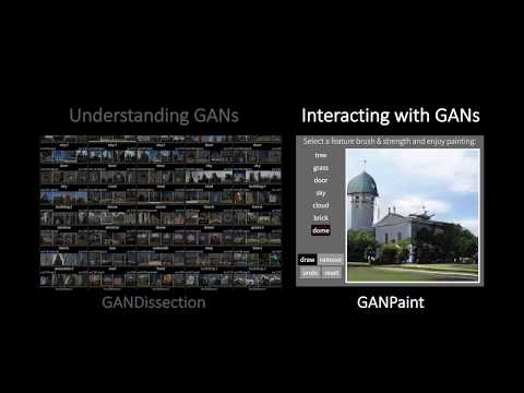
You can also play with very cool interactive demo on gandissect.res.ibm.com.

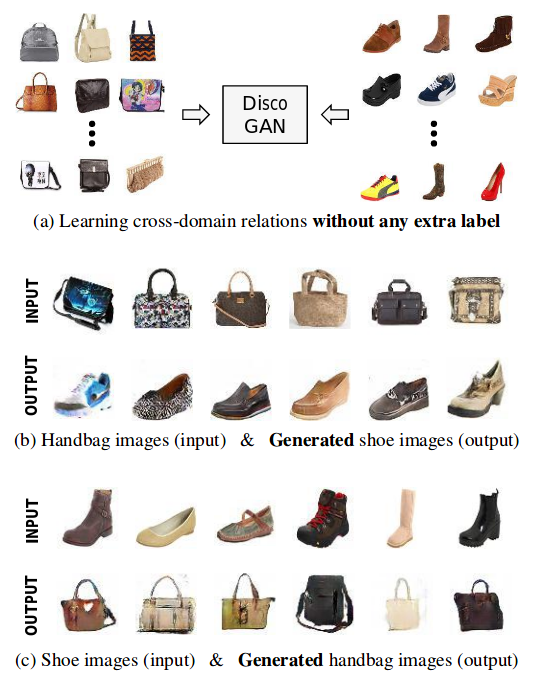
DiscoGAN: DiscoGAN has lot like CycleGAN, where DiscoGAN successfully transfers style from one domain to another while preserving key attributes such as orientation and face identity. Suppose we have collected two sets of images, one containing handbags and another containing only shoes. DiscoGAN trains on sets independently and learn how to map two domains without any extra label. So, we can convert a handbag into shoe which will have same color and any such attribute, all we need to pass DiscoGAN is a handbag. Difference between in DiscoGAN and CycleGAN is what losses are used to reconstruction. CycleGAN uses cycle consistency loss while DiscoGAN uses reconstruction loss separate for both domains.

pix2pixHD: Okay we have to stop somewhere, let stop with last mention to a type of conditional GAN to synthesize High-Resolution Image and Semantic Manipulation aka pix2pixHD. And results they sure don’t disappoint.

Further apologizes to remaining GAN family for not mentioning them in special mentions. Shall we do one more section special special mentions 😛?

Look at the progress from introducing GANs to the world in 2014 to worrying about dangerous impact on society caused by GAN in 2017, this speaks more than I can make you understand. And this is the story of GANs.

In next post, we will do something different. We will attempt to dissect any one or two papers. Any suggestions? So, let’s call our next adventure Fun of paper dissection. And further build a text recognizer application and deploy it for fun. A lot to come, a lot of fun!

Happy Learning!