Long-Short Term Memory and Gated Recurrent Unit

In this post, we will see if we can analyse the sentiment in reviews of movies on IMDB dataset.

All the codes implemented in Jupyter notebook in Keras, PyTorch, Flair and fastai.

All codes can be run on Google Colab (link provided in notebook).

Hey yo, but how?

Well sit tight and buckle up. I will go through everything in-detail.

Feel free to jump anywhere,

Preprocessing Text
Introduction to LSTM and GRU
Further Reading
Footnotes and Credits

Preprocessing Text

The data used in applications for nlp is messy, contains lot of noise. There are all sorts of preprocessing steps we need to carry to convert this messy data to useful data. Let’s look into some of the preprocessing steps.

Sentence: "<h2>I don't know about you but i'm feeling 22</h2>"

Remove HTML tags

Here is where Beautiful Soup comes to resuce.

def strip_html_tags(text):
    soup = BeautifulSoup(text, "html.parser")
    stripped_text = soup.get_text()
    return stripped_text

Input: <h2>I don't know about you but i'm feeling 22</h2>

Output: I don't know about you but i'm feeling 22

Remove accented characters

A simple example — converting é to e.

def remove_accented_chars(text):
    text = unicodedata.normalize('NFKD', text).encode('ascii', 'ignore').decode('utf-8', 'ignore')
    return text

Input: Sómě Áccěntěd těxt

Output: Some Accented text

Expanding Contractions

Contractions are shortened version of words or syllables. These shortened versions or contractions of words are created by removing specific letters and sounds. In case of English contractions, they are often created by removing one of the vowels from the word. Examples would be, do not to don’t and I would to I’d.

def expand_contractions(text, contraction_mapping=CONTRACTION_MAP):
    
    contractions_pattern = re.compile('({})'.format('|'.join(contraction_mapping.keys())), 
                                      flags=re.IGNORECASE|re.DOTALL)
    def expand_match(contraction):
        match = contraction.group(0)
        first_char = match[0]
        expanded_contraction = contraction_mapping.get(match)\
                                if contraction_mapping.get(match)\
                                else contraction_mapping.get(match.lower())                       
        expanded_contraction = first_char+expanded_contraction[1:]
        return expanded_contraction
        
    expanded_text = contractions_pattern.sub(expand_match, text)
    expanded_text = re.sub("'", "", expanded_text)
    return expanded_text

Input: I don't know about you but i'm feeling 22

Output: I do not know about you but i am feeling 22

Removing Special Characters and digits

Removing special character like @ which is often used in tweets, <, >, quotations, any other punctuations, etc can make text useful for further processing. Removing digits can be optional.

def remove_special_characters(text, remove_digits=True):
    pattern = r'[^a-zA-z0-9\s]' if not remove_digits else r'[^a-zA-z\s]'
    text = re.sub(pattern, '', text)
    return text

Input: I do not know about @you but i am feeling 22

Output: I do not know about you but i am feeling

Stemming

Stemming refers to a simpler version of lemmatization in which we mainly stemming just strip suffixes from the end of the word.

def stemmer_text(text):
    ps = nltk.porter.PorterStemmer()
    text = ' '.join([ps.stem(word) for word in text.split()])
    return text

Input: I do not know about you but i am feeling 22

Output: I do not know about you but i am feel 22

Lemmatization

Lemmatization is the task of determining that two words have the same root, despite their surface differences. For example, the words sang, sung, and sings are forms of the verb sing. The word sing is the common lemma of these words, and a lemmatizer maps from all of these to sing. Lemmatization is essential for processing morphologically complex languages like Arabic.

def lemmatize_text(text):
    text = nlp(text)
    text = ' '.join([word.lemma_ if word.lemma_ != '-PRON-' else word.text for word in text])
    return text

Input: I do not know about you but i am feel 22

Output: I do not know about you but i be feel 22

Removing Stopwords

These are usually words that end up having the maximum frequency if you do a simple term or word frequency in a corpus. Some examples of stopwords are a, an, the, and, of, is, etc.

def remove_stopwords(text, is_lower_case=False):
    tokens = tokenizer.tokenize(text)
    tokens = [token.strip() for token in tokens]
    if is_lower_case:
        filtered_tokens = [token for token in tokens if token not in stopword_list]
    else:
        filtered_tokens = [token for token in tokens if token.lower() not in stopword_list]
    filtered_text = ' '.join(filtered_tokens)    
    return filtered_text

Input: I do not know about you but i be feel 22

Output: not know feel 22

After we obtain clean text, we use any of the vectorization or embedding methods mentioned below to convert string to numbers.

Introduction to LSTM and GRU

A long time ago in a galaxy far, far away….

I-know-everything: Today we will be visiting a lot of concepts in field of NLP. I mean a lot. There will be a lot to take in so don’t get lost (in space).

I-know-nothing: I better pay attention then.

I-know-everything: Let me start with introduction to various vectorization and embeddings techniques and gradually we will move into LSTM and GRUs.

In the last post on RNNs we saw how neural networks only understand numbers and all we have as input is string of words which make up sentences, which make up paragraphs and eventually a document. Collection of such documents is called corpus. The text is converted to tokens using tokens and into numbers using vectorization/embeddings/numericalizations.

So, to convert the text we often take help of various techniques. Let’s visit them one by one.

Vectorization

Vectorization refers to the process of converting strings to numbers. These numbers which are then fed to neural networks to do their thing. There are various ways we can convert these strings into numbers. This process is also called feature extraction or feature encoding. In this techniques we will often encounter with the word Vocabulary, vocab is nothing but collection of unique words or characters depending on how we want.

We will make this concrete with example.

Example Sentence: The cat sat on the mat.

vocab_character : {T, h, e, c, a, t, s, o, n, m, .}

vocab_words : {The, cat, sat, on, the, mat, .}

If we had converted all the text to lower, new vocabulary would have been

vocab_character : {t, h, e, c, a, s, o, n, m, .}

vocab_words : {the, cat, sat, on, mat, .}

Notice, the repeated “the” is now gone. Hence, unique collection of words or characters.

Note: we will assume that our sentences will be lower case even though they may appear upper case.

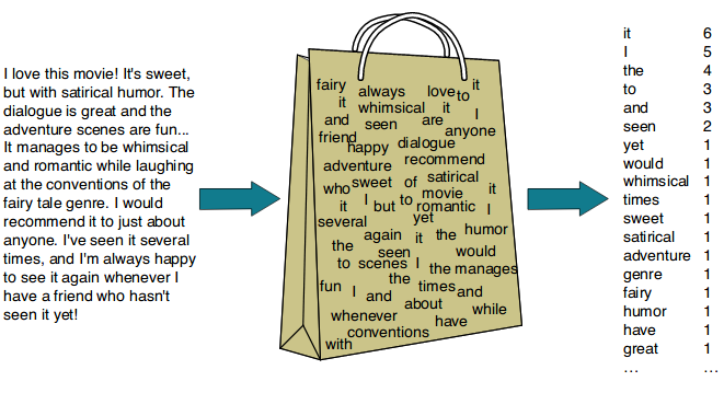
Bag-of-Words Model

This is one of the most simple and naive way to vectorize. As the name suggests, we are creating a bag of unique words. The simplest way to create a vocabulary is to bag unique words(characters).

Sentence 1: I came I saw

Sentence 2: I conquered

From these three sentences, our vocabulary is as follows:

{ I, came, saw, conquered }

Count Vectorizer

BoW Model learns a vocabulary from each document and model each document by counting the occurence of word in the document. This is done on top of Bag-of-Models. Here each word count is considered as feature vector. Count vectorizer works on Terms Frequency, i.e. counting the occurrences of tokens.

We will understand more clearly by example where each sentence is considered a document,

Sentence 1: I came I saw

Sentence 2: I conquered

From these three sentences, our vocabulary is as follows:

{ I, came, saw, conquered }

To get our bags of words using count vectorizer, we count the number of times each word occurs in each sentence. In Sentence 1, “I” appears twice, and “came” and “saw” each appear once, so the feature vector for Sentence 1 is:

Sentence 1: { 2, 1, 1, 0 }

Similarly, the features for Sentence 2 are: { 1, 0, 0, 1 }

TF-IDF Vectorizer

Count Vectorizer tend to give higher score to more dominant words from the document but they may not contain “informational content” as much as rarer but domain specific words. For example, “I” from above example. Hence, we introduce TF-IDF. TF-IDF stands for term frequency-inverse document frequency. It gives a score as to how important a word is to the document in a corpus. TF-IDF measures relevance, not frequency. Word counts are replaced with TF-IDF scores across the whole corpus.The scores have the effect of highlighting words that are distinct (contain useful information) in a given document. The IDF of a rare term is high, whereas the IDF of a frequent term is likely to be low.

Term Frequency: is a scoring of the frequency of the word in the current document.
Inverse Document Frequency: is a scoring of how rare the word is across documents.

TF(t) = Number of times t appears in document / Total number of terms in document

IDF(t) = log(Total number of documents / Number of documents with term t in it)

TF-IDF(t) = TF(t) * IDF(t)

Let’s look at our example,

Document 1 consists of Sentence 1:

Term Frequency of Document 1 = {I: 2, came:1, saw: 1}

Term Frequency of Document 2 = {I: 1, conquered: 1}

Let’s calculate TF-IDF(“conquered”) ,

TF(“conquered”) for Document 1 = 0/4

TF(“conquered”) for Document 2 = 1/2

IDF(“conquered”) = log(2/1)

TF-IDF(“conquered”) for Document 1 = (0/4) * log(2/1)

TF-IDF(“conquered”) for Document 2 = (1/2) * log(2/1)

We get different weightings for same word.

N-gram Models

N-gram is contiguous sequence of n-items. Remember how using BoW we count occurrence of single word. Now, what if instead of using single word we used 2 consecutive words as construct bag-of-models from this model, n=2, also called bigram. We add the count based on the vocab used to construct a feature vector for n-gram.

1-gram model (unigram), the new vocab will be { I, came, saw, conquered} same as BoW model vocabulary.

2-gram model (bigram), the new vocab will be { I came, came I, I saw, I conquered}

3-gram model (trigram), the new vocab will be {I came I, came I saw}

BoW can be considered as special case of n-gram model with n=1.

Adding features of higher n-grams can be helpful in identifying that a certain multi-word expression occurs in the text.

Limitations of Bag-of-Words Model

Vocabulary

The size of vocabulary requires careful design, most specifically in order to manage the size. The misspelling like come, cmoe will be considered as seperate words which can lead to increase in vocabulary.

Sparsity

Sparse representations are harder to model both for computational reasons (space and time complexity). There will be a lot of zeros as input vectors will be one hot encoded of vocabulary size.

Ordering

Discarding word order ignores the context, and in turn meaning of words in the document (semantics). Context and meaning can offer a lot to the model, that if model could tell the difference between the same words differently arranged (“this is interesting” vs “is this interesting”), synonyms (“old bike” vs “used bike”), and much more. This is one of the crucial drawbacks of using BoW models.

Embeddings

Embeddings are the answer to mitigate the drawbacks of BoW model. Embeddings take into account the context and semantic meanings of words by producing a n-dimensional vector corresponding to that word. This vector captures the semantic meaning. We will look into some of the popular ways of creating embeddings using different methods.

Word2Vec

Ahh, the title, Word2Vec, converts a word to vector. Mikilov et al developed the word2vec toolkit that allows to use pretrained embeddings. But how? Word2vec is similar to an autoencoder, encoding each word in a vector. Word2Vec trains words against other words that neighbor them in the input corpus. Word2Vec consists of 3-layer neural network (not very deep) i.e. input layer, hidden layer and output layer. Depending on which model (skip-gram or cbow), we feed in word and train to predict neighbouring words or feed neighbouring words and train to predict missing word. Once we obtain trained model, we remove last output layer and when we input a word from vocabulary, output given by hidden layer will be “embedding of the input word”.

If the network is given enough training data (tens of billions of words), it produces word vectors with intriguing characteristics. Words with similar meanings appear in clusters, and clusters are spaced such that some word relationships, such as analogies, can be reproduced using vector math. The famous example is that, with highly trained word vectors, “king - man + woman = queen.” Patterns such as “Man is to Woman as Brother is to Sister” can be generated through algebraic operations on the vector representations of these words such that the vector representation of “Brother” - ”Man” + ”Woman” produces a result which is closest to the vector representation of “Sister” in the model. Such relationships can be generated for a range of semantic relations (such as Country–Capital) as well as syntactic relations (e.g. present tense–past tense). A similar example of the result of a vector calculation vec(“Madrid”) - vec(“Spain”) + vec(“France”) is closer to vec(“Paris”) than to any other word vector.

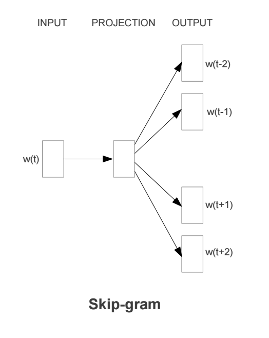
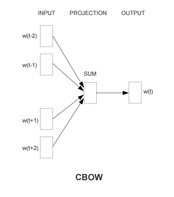
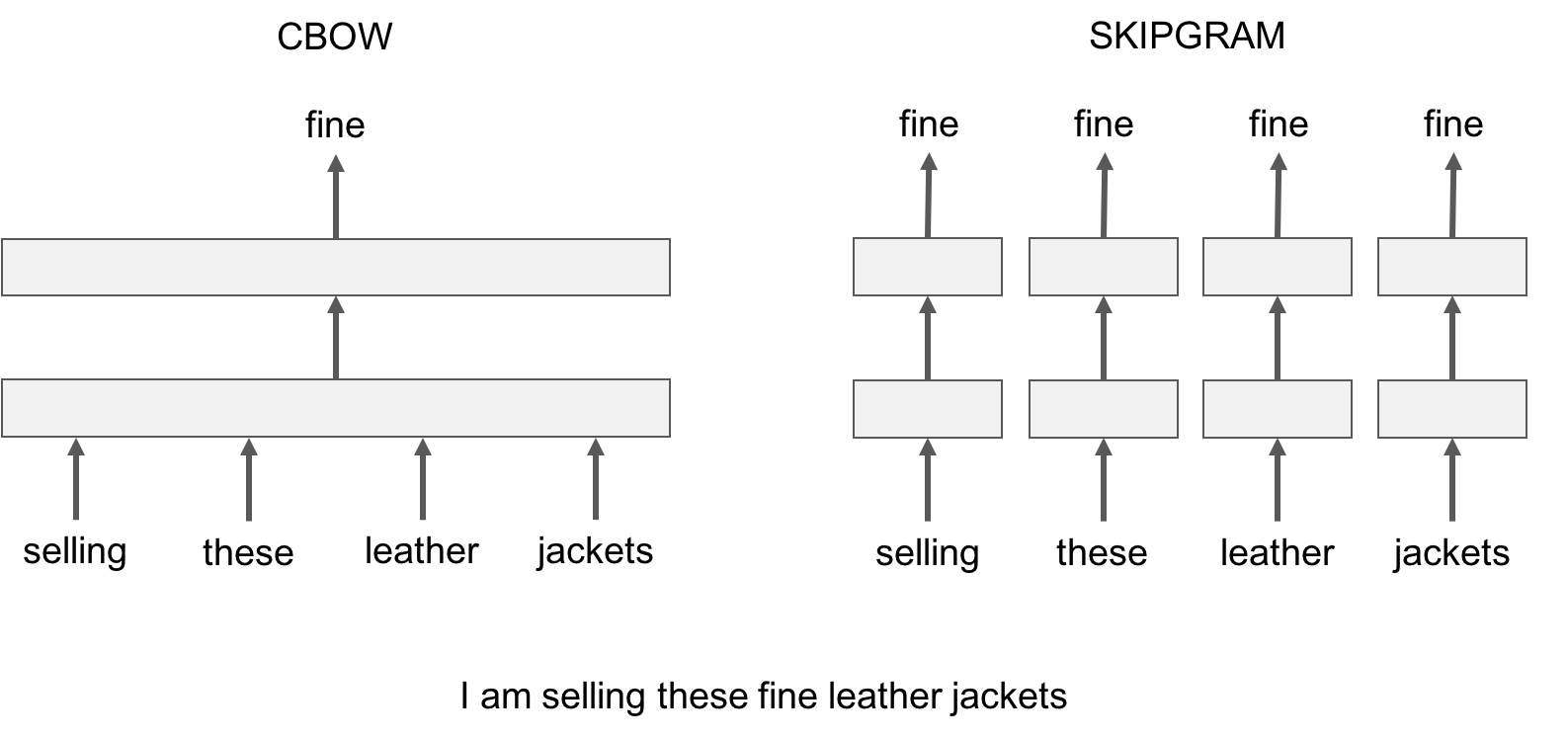
It comes in two flavors, the Continuous Bag-of-Words model (CBOW) and the Skip-Gram model. Algorithmically, these models are similar, except that CBOW predicts target words (e.g. ‘mat’) from source context words (‘the cat sits on the’), while the skip-gram does the inverse and predicts source context-words from the target words.

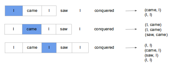
Skip-gram Model

Skip-gram model predicts context (surrounding) words given the current word. The training objective is to learn word vector representations that are good at predicting the nearby words. To understand what that means, lets consider example shown below.

Here we consider the window size = 2, window size refers to the number of words to be looked on either side of focus or input word. The highlighted blue color word is input and it produces training samples depending on context words.

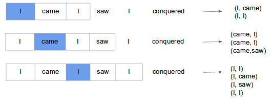
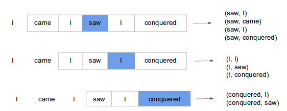
The pairs to right are training samples i.e (context, target) pairs. The training of skip-gram will take one-hot vector input on vocabulary and outputs a probability after applying Hierarchical softmax that the particular word is output given the input word. Given enough input vectors, model learns that there is high probability that when “San” is given as input, “Francisco” or “Jose” is more likely than “York”. Skip-gram treats each context-target pair as a new observation, and this tends to do better when we have larger datasets.

CBOW Model

Continuous bag of words (CBOW) model predicts the current word based on several surrounding words. The training objective is to learn word vector representations that are good at predicting missing word given the context words.

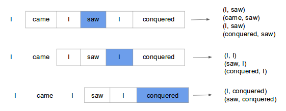
The pairs to right are training samples i.e. (context, target) pairs. It’s like all the pairs from above Skip-gram training samples are inverted. That’s exactly how it is. CBOW smoothes over a lot of the distributional information (by treating an entire context as one observation). For the most part, this turns out to be a useful thing for smaller datasets. CBOW is faster while skip-gram is slower but does a better job for infrequent words.

Training Tricks

Word2Vec uses some tricks in training. We will look at some of them.

Subsampling Frequent Words

We have seen how training samples are created. In very large corpora, the most frequent words can easily occur hundreds of millions of times (e.g.,“in”, “the”, and “a”). Such words usually provide less information value than the rare words and being the most common word it occurs pretty much everywhere. So, how to learn a good vector for the word “the”? This where the authors propose a subsampling method for frequent words. The idea to change the vector representation of frequent words gradually. To counter the imbalance between the rare and frequent words, authors used a simple subsampling approach: each word \(\mathbf{w_{i}}\) in the training set is discarded with probability computed by the formula \(P(\mathbf{w_i}) = 1 - \sqrt{\frac{t}{\mathbf{f(\mathbf{w}_i)}}}\) where \(\mathbf{f(\mathbf{w}_i)}\) is the frequency of word \(\mathbf{w_i}\) and t is a chosen threshold, typically around \(10^{-5}\).

Hierarchical Softmax

The traditional softmax is very computationally expensive especially for large vocabulary size, typically for vocabulary size of V the order is O(V) which is often of size (\(10^{5}\) - \(10^{7}\) terms), but hierarchical softmax reduces the computation to O(log(V)). Replacing a softmax layer with H-Softmax can yield speedups for word prediction tasks of at least 50x. The hierarchical softmax uses a binary tree representation of the output layer with the \(\mathbf{W}\) words a sits leaves and, for each node, explicitly represents the relative probabilities of its child nodes. As binary tree(remember binary search) is involved, the output will look if target word is first half or second half of tree and so on till it reaches a leaf of tree where the target sits. This reduces the complexity equal to the depth of tree instead of classifying looking through whole vocabulary through softmax where we sum over all vocabulary in the denominator. This is one idea for speeding up softmax calculation.

To look more about hierarchical softmax, here is awesome video explaination by Hugo Larochelle.

Negative Sampling

This methods provides a work around to let us keep traditional softmax and still achieve a less computationally expensive model. As we have seen in loss functions in previous posts, the maximum likelihood principle maximises the probability of \(\mathbf{w_t}\) (“target”) given the context \(\mathbf{h}\), i.e. \(\mathbf{J_{ML}} = \log_{}P(\mathbf{w_t}\mid\mathbf{h})\). With negative sampling, we are instead going to randomly select just a small number of “negative” words (k = 7) to update the weights for. Here negative words are the words other than the context words with respect to focus or input word. In this case, a positive example would be (I, saw) and negative sample would be (I, book) or (I, king), picking a random word from vocabulary. The authors propose that selecting 5-20 words works well for smaller datasets, and 2-5 words for large datasets. Negative samples are selected using “unigram distribution”, where most frequent words are more likely to be selected. For e.g. the probability of picking word “saw” is the total number of times the word occurs in the corpus divided by the total number of words in the corpus. Authors found that word counts raised to power (3/4) gave good empirical results than power of 1. This one has the tendency to increase the probability for less frequent words and decrease the probability for more frequent words like “the, is, of”. The new objective is maximized when the model assigns high probabilities to the real words, and low probabilities to noise(negative) words. It is binary classification problem on k+1 (context, target) pairs it contains k negative samples and 1 positive samples where task is to predict is each of (context, target) pair is positive sample or not.

For more on negative sampling derivation, look into very short paper by Goldberg and Levy.

Sebastian Ruder has great in-depth discussion of various sampling and softmax classifiers in this blog, definitely worth a look.

There are many hyperparmamerters while training the algorithm and the most crucial decisions that affect the performance are the choice of the model architecture, the size of the vectors, the subsampling rate, and the size of the training window. One of the biggest challenges with Word2Vec is how to handle unknown or out-of-vocabulary (OOV) words and morphologically similar words. This can particularly be an issue in domains like medicine where synonyms and related words can be used depending on the preferred style of radiologist, and words may have been used infrequently in a large corpus. If the word2vec model has not encountered a particular word before, it will be forced to use a random vector, which is generally far from its ideal representation.

Here is one example of projecting the learned embedding in 2d space using tSNE.

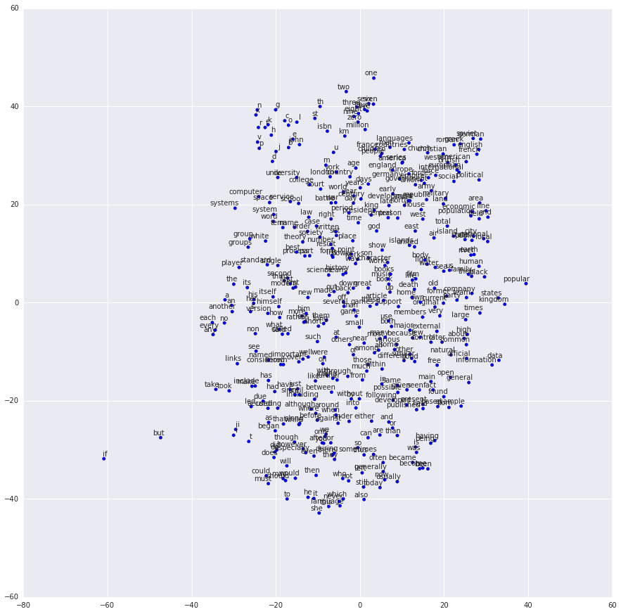
Here we can see, the words like two, million, three are group together and words like he, she, it are clustered together and many other clusters are formed.

GloVe

While the word2vec serendipitous discovered that the words semantically similar tend to be closer as shown in figure above. The authors of GloVe paper show how that the ratio of the co-occurrence probabilities of two words is what contains information and aim to encode this information as vector differences.

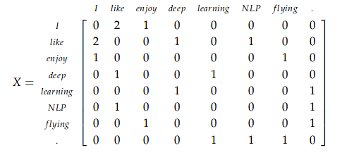
Let us first look into what is co-occurence matrix. Consider three sentences with window size = 1. Then the co-occurence matrix X will be,

I enjoy flying.
I like NLP.
I like deep learning.

Authors propose a training objective J that directly aims to minimise the difference between the dot product of the vectors of two words and the logarithm of their number of co-occurrences,

\[J = \sum_{i,j=1}^{V}f(\mathbf{X_{ij}})(\mathbf{w_{i}^{T}}\mathbf{\hat{w}_{j}} + \mathbf{b_i} + \mathbf{\hat{b}_{j}} - \log_{}{\mathbf{X_{ij}}})^2\]

where \(\mathbf{w_{i}}\) and \(\mathbf{b_{i}}\) are word vector and bias of word i, \(\mathbf{\hat{w}_{j}}\) and \(\mathbf{\hat{b}_{j}}\) are context word vector and bias of word j, \(\mathbf{X}\) is the co-occurence matrix and \(\mathbf{X_{ij}}\) is the number of times word i occurs in the context of word j, and f is a weighting function that assigns relatively lower weight to rare and frequent co-occurrences. It is defined as:

\[f(x) = \begin{cases} (\frac{x}{\mathbf{x_{max}}})^\alpha & x < \mathbf{x_{max}} \\ 1 & otherwise \end{cases}\]

where \(\mathbf{x_{max}}\) and \(\alpha\) are hyperparameters, authors found \(\mathbf{x_{max}}\)=100 and \(\alpha\)=0.75 showing good performance.

fastText

fastText is a library created by the Facebook Research Team for efficient learning of word representations and sentence classification. The key difference between fastText and Word2Vec is the use of n-grams. In fastText each word is represented as bag of character of n-gram. For e.g. the word where and n=3 as an example, it will represented by the character n-grams: <wh, whe, her, ere, re> and special sequence , < and > are added at begining and end of the words to distinguish prefixes and suffixes from other character sequences i.e. , corresponding to word her can also be part of vocabulary and will be different from tri-gram "her" from where. At each training step in fastText, the mean of the target word vector and its component n-gram vectors are used for training. The adjustment that is calculated from the error is then used uniformly to update each of the vectors that were combined to form the target. This adds a lot of additional computation to the training step. At each point, a word needs to sum and average its n-gram component parts. The trade-off is a set of word-vectors that contain embedded sub-word information. These vectors have been shown to be more accurate than Word2Vec vectors by a number of different measures.

fastText offers a better luxury in handling OOV words as it can construct the vector for a OOV word from its character n grams even if word doesn’t appear in training corpus. Both Word2vec and Glove can’t.

We will look into CoVe, ELMo, ULMFit, GPT, BERT and GPT-2 models in the post on Transfer Learning in NLP.

I-know-nothing: So, what I understand is that we can use any of these techniques above to convert individual words into numbers. But aren’t embeddings are biased. Can we talk a little about bias in embeddings?

I-know-everything: Haha, you caught me. That’s absolutely right. And embedding learned are defintely biased. So to give example, if we give a relation such as Man:Doctor :: Woman:?, then the learned embeddings will with almost certainity predict the answer to be Nurse (What a biasist) or Man:Computer Programmer::Woman:Homemaker. The community has proposed several ways of “debiasing embeddings”. All the pretrained embedding from above acquire stereotypical human biases from the text data they are trained on i.e. word embeddings can reflect gender, ethinicity, age, sexual orientation, and other biases of the text data used to train the model.

Debiasing Embeddings

We will understand a simple gender debiasing algorithm outlined in this paper, some other biases like religion or racial can also be used in similar way.

Identify the gender space

To identify a gender direction g, we aggregate across multiple pair comparisons by combining several comparisons like \(\vec{man}\) - \(\vec{woman}\), \(\vec{he}\) - \(\vec{she}\), \(\vec{male}\) - \(\vec{female}\), etc which largely captures gender in the embedding. This direction helps us to quantify direct and indirect biases in words and associations.

Neutralize

For every word that is not definitional, project to get rid of bias. These words can be occupational like babysit, doctor, nurse, etc. Neutralize ensures that gender neutral words are zero in the gender subspace.

Equalize pairs

Equalize perfectly equalizes sets of words outside the subspace and there by enforces the property that any neutral word is equidistant to all words in each equality set. For instance, if {grandmother, grandfather} and {guy, gal} were two equality sets, then after equalization babysit would be equidistant to grandmother and grandfather and also equidistant to gal and guy, but presumably closer to the grandparents and further from the gal and guy. This is suitable for applications where one does not want any such pair to display any bias with respect to neutral words.

To reduce the bias in an embedding, we change the embeddings of gender neutral words, by removing their gender associations. For instance, nurse is moved to to be equally male and female in the direction g. In addition, we find that gender-specific words have additional biases beyond g. For instance, grandmother and grandfather are both closer to wisdom than gal and guy are, which does not reflect a gender difference. On the other hand, the fact that baby sit is so much closer to grandmother than grandfather(more than for other gender pairs) is a gender bias specific to grandmother. By equating grandmother and grandfather outside of gender, and since we’ve removed g from babysit,both grandmother and grandfather and equally close to baby sit after debiasing. By retaining the gender component for gender-specific words, we maintain analogies such as she:grandmother:: he:grandfather.

As an example, consider the analogy puzzle, he to doctor is as she to X. The original embedding returns X = nurse while the hard-debiased embedding finds X = physician.

To further look into this topic, I am adding link to few papers here, here, here, here, here, here and here

Now, having looked at embeddings, we will move into new architectures which we will introduce to overcome the shortcomings in RNN.

Exploding and Vanishing Gradients

With conventational Back-Propogation through time(BPTT) which we looked in context of RNN in our last post, error signals(or gradients) “flowing backwards in time” tend to blow up(explode) or vanish. We can understand exploding and vanishing effects through two examples, one from compounding where the amount keeps multiplying and turn out to be very large amount and similarly if a gambler loses 3 cents for every dollar, the amount keeps multiplying and becomes less and less, eventually making gambler bankrupt. Similarly, large gradients keep multiplying through backpropagation through time backwards result in very large number and vice-versa.

Long-term dependency example of is, “I studied Spainish in my class. So, the other day I visited Spain. It was an amazing experience. We enjoyed a lot. We ran up and down the road. We played football and put many such sentences in between. But the coming from English background, we had difficulty conversing fluently in ….” If we ask RNN to fill in the blank with appropriate word, the word should be “Spanish” but as the relation between studying and conversing is far away, RNN will not be able to predict the correct word.

LSTM Network

LSTM or Long Short Term Memory introduced by Hochreiter & Schmidhuber - a speical kind of RNN- capable of learning long-term dependencies. LSTMs are explicitly designed to avoid the long-term dependency problem.

The best explaination step-by-step is given by Christopher Olah in his wonderful blog on Understanding LSTM Networks.

I will just write the equations and maybe explain a bit. But his blog covers it all step-by-step. So, let’s begin.

Let’s start with mathematical formulation of LSTM units. It’s going to be scary, be warned.

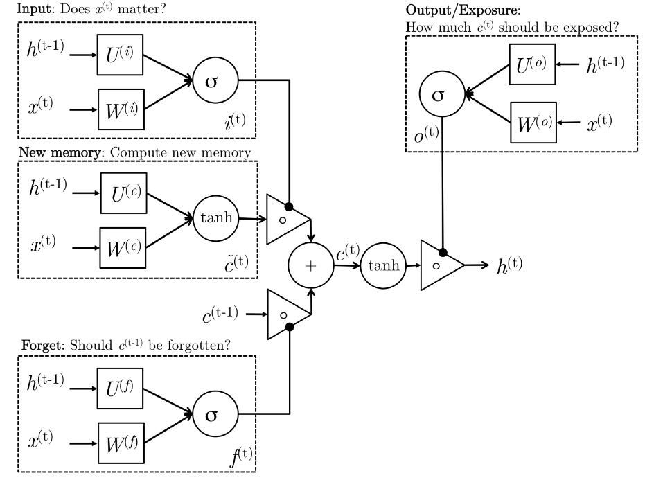
\[\begin{aligned} i^{(t)} & = \sigma(W^{(i)}x^{(t)} + U^{(i)}h^{(t-1)}) & \text{(Input Gate)}\\ f^{(t)} & = \sigma(W^{(f)}x^{(t)} + U^{(f)}h^{(t-1)}) & \text{(Forget Gate)}\\ o^{(t)} & = \sigma(W^{(o)}x^{(t)} + U^{(o)}h^{(t-1)}) & \text{(Output Gate)}\\ \tilde{c}^{(t)} & = \sigma(W^{(c)}x^{(t)} + U^{(c)}h^{(t-1)}) & \text{(New Memory cell)}\\ c^{(t)} & = f^{(t)} \cdot \tilde{c}^{(t-1)} + i^{(t)} \cdot \tilde{c}^{(t)} & \text{(Final Memory cell)}\\ h^{(t)} & = o^{(t)} \cdot tanh(c^{(t)})\\ \end{aligned}\]

Here is an illustration explaining what is going on in above equations.

So, what is really going on?

Let’s go step by step through the architecture. The LSTM have the ability to remove or add information to the cell state (\(c^{(t)}\)), carefully regulated by structures called gates.

New memory generation

We use the input word \(x^{(t)}\) and the past hidden state \(h^{(t-1)}\) to generate new memory state \(\tilde{c}^{(t)}\) which includes some information about input word \(x^{(t)}\).

Input Gate

We see that the new memory generation stage doesn’t check if the new word is even important before generating the new memory – this is exactly the input gate’s function. The input gate uses the input word and the past hidden state to determine whether or not the input is worth preserving and thus is used to gate the new memory. It thus produces \(i^{(t)}\) as an indicator of this information.

Forget Gate

This gate is similar to the input gate except that it does not make a determination of usefulness of the input word – instead it makes an assessment on whether the past memory cell is useful for the computation of the current memory cell. Thus, the forget gate looks at the input word and the past hidden state and produces \(f^{(t)}\). The sigmoid layer outputs numbers between zero and one, describing how much of each component should be let through. A value of zero means “let nothing through,” while a value of one means “let everything through!” A 1 represents “completely keep this” while a 0 represents “completely get rid of this.”

Final Memory Generation

This stage first takes the advice of the forget gate \(f^{(t)}\) and accordingly forgets the past memory \(c^{(t-1)}\). Similarly, it takes the advice of the input gate \(i^{(t)}\) and accordingly gates the new memory \(\tilde{c}^{(t)}\). It then sums these two results to produce the final memory \(c^{(t)}\).

Output Gate

It’s purpose is to separate the final memory from the hidden state. The final memory \(c^{(t)}\) contains a lot of information that is not necessarily required to be saved in the hidden state. Hidden states are used in every single gate of an LSTM and thus, this gate makes the assessment regarding what parts of the memory \(c^{(t)}\) needs to be present in the hidden state \(h^{(t)}\). The signal it produces to indicate this is \(o^{(t)}\) and this is used to gate the pointwise tanh of the memory.

If any Pokemon fans out there, check this awesome example explaination provided by Edwin Chen on his blog of Exploring LSTMs.

GRU Network

Having learnt what LSTM does, we try to minimze the number of equations/gates and instead of forget gate, input gate and output gate, we just introduce two gates, Update gate and Reset Gate in GRU (Gated Recurrent Unit).

And the scariness continues.

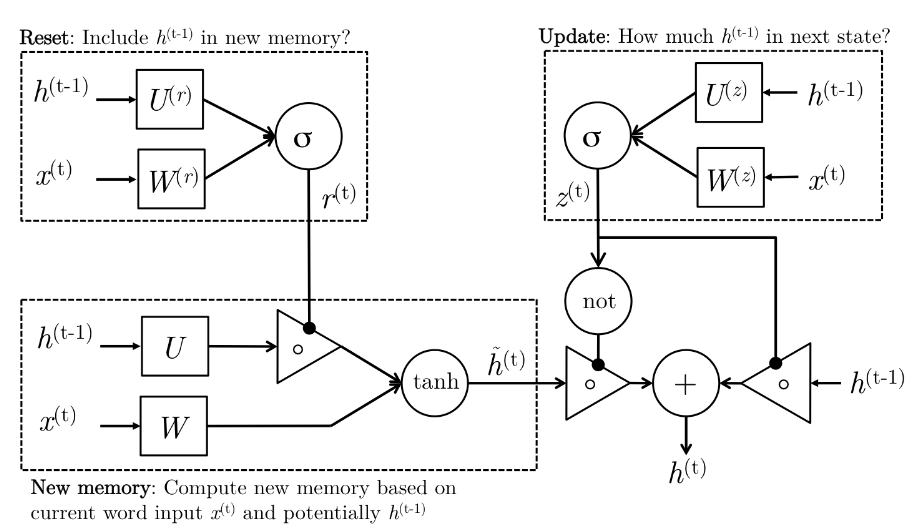
\[\begin{aligned} z^{(t)} & = \sigma(W^{(z)}x^{(t)} + U^{(z)}h^{(t-1)}) & \text{(Update Gate)}\\ r^{(t)} & = \sigma(W^{(r)}x^{(t)} + U^{(r)}h^{(t-1)}) & \text{(Reset Gate)}\\ \tilde{h}^{(t)} & = tanh(r^{(t)} \cdot U^{(t)}h^{(t-1)} + Wx^{(t)} ) & \text{(New Memory)}\\ h^{(t)} & = (1-z^{(t)}) \cdot \tilde{h}^{(t)} + z^{(t)} \cdot \tilde{h}^{(t-1)} & \text{(Hidden State)}\\ \end{aligned}\]

Here is an illustration explaining what is going on in above equations.

So what is going on again?

New Memory Generation

A new memory \(\tilde{h}^{(t)}\) is the consolidation of a new input word \(x^{(t)}\) with the past hidden state \(h^{(t-1)}\). Anthropomorphically, this stage is the one who knows the recipe of combining a newly observed word with the past hidden state \(h^{(t-1)}\) to summarize this new word in light of the contextual past as thevector ̃\(\tilde{h}^{(t)}\).

Reset Gate

The reset signal \(r^{(t)}\) is responsible for determining how important \(h^{(t-1)}\) is to the summarization \(\tilde{h}^{(t)}\). The reset gate has the ability to completely diminish past hidden state if it finds that \(h^{(t-1)}\) is irrelevant to the computation of the new memory.

Update Gate

The update signal \(z^{(t)}\) is responsible for determining how much of \(h^{(t-1)}\) should be carried forward to the next state. For instance, if \(z^{(t)} \approx\) 1, then \(h^{(t-1)}\) is almost entirely copied out to \(h^{(t)}\). Conversely, if \(z^{(t)} \approx\) 0, then mostly the new memory ̃\(\tilde{h}^{(t)}\) is forwarded to the next hidden state.

Hidden State

The hidden state \(h^{(t-1)}\) is finally generated using the past hidden input \(h^{(t-1)}\) and the new memory generated \(\tilde{h}^{(t)}\) with the advice of the update gate.

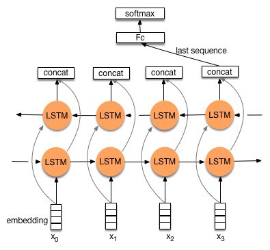
Bidirectional LSTM Network

These are just the derivation of LSTM where we stack two lstm on top of each other. One LSTM runs a forward pass, while the another LSTM runs a backward pass and finally both the outputs are concatenated.

What can we do with help of these networks? Movie Reviews? Calling IMDB…

Let’s see at nlpprogess what is the current state-of-the-art in sentiment analysis.

Model	Accuracy	Paper
ULMFit	95.4	Universal Language Model Fine-tuning for Text Classification
Block-sparse LSTM	94.99	GPU Kernels for Block-Sparse Weights
oh-LSTM	94.1	Supervised and Semi-Supervised Text Categorization using LSTM for Region Embeddings
Virtual adversarial training	94.1	Adversarial Training Methods for Semi-Supervised Text Classification
BCN+Char+CoVe	91.8	Learned in Translation: Contextualized Word Vectors

So, let’s use these network to see how well do they classify movie reviews. We will handpick some of the reviews and give sentiment as predicted by our trained model.

"This movie is a disaster within a disaster film. It is full of great action scenes, which are only meaningful if you throw away all sense of reality. Let's see, word to the wise, lava burns you; steam burns you. You can't stand next to lava. Diverting a minor lava flow is difficult, let alone a significant one. Scares me to think that some might actually believe what they saw in this movie.<br /><br />Even worse is the significant amount of talent that went into making this film. I mean the acting is actually very good. The effects are above average. Hard to believe somebody read the scripts for this and allowed all this talent to be wasted. I guess my suggestion would be that if this movie is about to start on TV ... look away! It is like a train wreck: it is so awful that once you know what is coming, you just have to watch. Look away and spend your time on more meaningful content."

Prediction: [0.99533975 0.00466027] -> 99% Negative

"Five medical students (Kevin Bacon, David Labraccio; William Baldwin, Dr. Joe Hurley; Oliver Platt, Randy Steckle; Julia Roberts, Dr. Rachel Mannus; Kiefer Sutherland, Nelson) experiment with clandestine near death & afterlife experiences, (re)searching for medical & personal enlightenment. One by one, each medical student's heart is stopped, then revived.<br /><br />Under temporary death spells each experiences bizarre visions, including forgotten childhood memories. Their flashbacks are like children's nightmares. The revived students are disturbed by remembering regretful acts they had committed or had done against them. As they experience afterlife, they bring real life experiences back into the present. As they continue to experiment, their remembrances dramatically intensify; so much so, some are physically overcome. Thus, they probe & transcend deeper into the death-afterlife experiences attempting to find a cure.<br /><br />Even though the DVD was released in 2007, this motion picture was released in 1990. Therefore, Kevin Bacon, William Baldwin, Julia Roberts & Kiefer Sutherland were in the early stages of their adult acting careers. Besides the plot being extremely intriguing, the suspense building to a dramatic climax & the script being tight & convincing, all of the young actors make \"Flatliners,\" what is now an all-star cult semi-sci-fi suspense. Who knew 17 years ago that the film careers of this young group of actors would skyrocket? I suspect that director Joel Schumacher did."

Prediction: [0.7998832 0.20011681] -> 80% Negative -> Misprediction

"All in all, this is a movie for kids. We saw it tonight and my child loved it. At one point my kid's excitement was so great that sitting was impossible. However, I am a great fan of A.A. Milne's books which are very subtle and hide a wry intelligence behind the childlike quality of its leading characters. This film was not subtle. It seems a shame that Disney cannot see the benefit of making movies from more of the stories contained in those pages, although perhaps, it doesn't have the permission to use them. I found myself wishing the theater was replaying \"Winnie-the-Pooh and Tigger too\", instead. The characters voices were very good. I was only really bothered by Kanga. The music, however, was twice as loud in parts than the dialog, and incongruous to the film.<br /><br />As for the story, it was a bit preachy and militant in tone. Overall, I was disappointed, but I would go again just to see the same excitement on my child's face.<br /><br />I liked Lumpy's laugh...."

Prediction: [0.02207627 0.9779237 ] -> 98% Positive

In next post, we will look into the most exicting topic in NLP, Power of Transfer Learning in NLP.

Happy Learning!