Object Detection

In this post, we will try to answer to the question, “Can computers identify and locate the objects better than humans?”

All the codes implemented in Jupyter notebook in Keras, PyTorch, Tensorflow, fastai and Demos.

All codes can be run on Google Colab (link provided in notebook).

Hey yo, but how?

Well sit tight and buckle up. I will go through everything in-detail.

Feel free to jump anywhere,

Loss Functions
- Classification Loss
- Regression Loss
Introduction to Object Detection
- Viola-Jones
- OverFeat
- R-CNN
- Fast R-CNN
- Faster R-CNN
- R-FCN
- SSD
- YOLO
  - YOLOv1
  - YOLOv2
  - YOLOv3
- RetinaNet
- Backbones
  - MobileNet
  - ResNeXt
  - FPN
Recap
Further Reading
Footnotes and Credits

Loss Functions

Loss functions are the heart of deep learning algorithms (in case you are wondering, backprop the soul). Loss functions tells the model how good the model is at particular task. Depending on the problem to solve, almost all model aim to minimize the loss. Also, did you notice one thing in particular about loss functions and non-linear functions, they are all “differentiable functions”. Yes, we may also call deep learning as “differentiable programming”. As there is No Free Lunch theorem in machine learning, which states that no one particular model can solve all the problems. Similarly, there is also no one particular loss function which when minimized(or maximize) will solve every task. If we make any changes to our model in hope(trying different hyperparameters) of creating better model, loss function will tell if we’re getting better model than previous model trained. If predictions of the model are totally off, loss function will output a higher number. If they’re pretty good, it’ll output a lower number. Designing loss functions to solve our particular task is one of the critical steps in deep learning, if we choose a poor error(loss) function and obtain unsatisfactory results, the fault is ours for badly specifying the goal of the search. (Choose wisely)

Loss function is defined in Deep Learning book as,

The function we want to minimize or maximize is called the objective function or criterion. When we are minimizing it, we may also call it the cost function, loss function, or error function.

There are lot many loss functions. But, broadly we can classify loss functions into two categories.

Classification Loss

As the name suggests, this loss will help with any task which requires classification. We are given k categories and our job is to make sure our model is good job in classifying x number of examples in k categories. An example from ImageNet competition, we are given 1.2 million images of 1000 different categories, and our task it to classify each given image into one of the 1000 categories.

Cross Entropy Loss

Cross-entropy loss is often simply referred to as “cross-entropy,” “logarithmic loss,” “logistic loss,” or “log loss” for short. Cross-entropy can be interpreted through two lens. One through information theory and other through probabilistic view.

Information theory view

The entropy rate of a data source means the average number of bits per symbol needed to encode it without any loss of information. Entropy of probability distribution p is given by \(H(p) = -\sum_{i}^{}p(i)\log_{2}{p(i)}\). Let p be the true distrubtion and q be the predicted distribution over our labels, then cross entropy of both distribution is defined as. \(H(p, q) = -\sum_{i}^{}p(i)\log_{2}{q(i)}\). It looks like pretty similar to equation of entropy above but instead of computing log of true probability, we compute log of predicted probability distribution.

The cross-entropy compares the model’s prediction with the label which is the true probability distribution. Cross entropy will grow large if predicted probability for true class is close to zero. But it goes down as the prediction gets more and more accurate. It becomes zero if the prediction is perfect i.e. our predicted distribution is equal to true distribution. KL Divergence(relative entropy) is the extra bit which exceeds if we remove entropy from cross entropy.

Aurélien Géron explains amazingly how entropy, cross entropy and KL Divergence pieces are connected in this video.

Probabilistic View

The output obtained from last softmax(or sigmoid for binary class) layer of the model can be interpreted as normalized class probabilities and we are therefore minimizing the negative log likelihood of the correct class or we are performing Maximum Likelihood Estimation (MLE).

As David Silver would like to say, let’s make it concrete with example. For example consider we get an output of [0.1, 0.5, 0.4] (cat, dog, mouse) where the actual or expected output is [1, 0, 0] i.e. it is a cat. But our model predicted that given input has only 10% probability of being a cat, 50% probability of being dog and 40% of chance being a mouse. This being a multi-class classification, we can calculate the cross entropy using the formula for \(\mathbf{L_{mce}}\) below.

Another example for binary class can be as follows. The models outputs [0.4, 0.6] (cat, dog) whereas the input image is a cat i.e. actual output is [1, 0]. Now, we can use \(\mathbf{L_{bce}}\) from below to calculate the loss and backpropgate the error and tell the model to correct its weight so as to get the output correct next time.

There are two different types of cross entropy functions depending on number of classes to classify into.

Binary Classification

As name suggests, there will be binary(two) classes. If we have two classes to classify our images into, then we use binary cross entropy. Cross entropy loss penalizes heavily the predictions that are confident but wrong. Suppose, \(\mathbf{\hat{y}}\) is our predicted output by the model and \(\mathbf{y}\) is target(actual or original) value. For M example, binary cross entropy can be forumlated as,

\[\begin{aligned} \mathbf{L_{bce}} = - \frac{1}{M}\sum_{i=1}^{M}(\mathbf{y_{i}}\log_{}{\mathbf{\hat{y}_{i}}} + (1-\mathbf{y}_{i})\log_{}{(1-\mathbf{\hat{y}_{i}})}) \end{aligned}\]

Multi-class Classification

As name suggests, if there are more than two classes that we want our images to be classified into, then we use multi-class classification error function. It is used as a loss function in neural networks which have softmax activations in the output layer. The model outputs the probability the example belonging to each class. For classifying into C classes, where C > 2, multi-class classification is given by,

\[\begin{aligned} \mathbf{L_{mce}} = - \sum_{c=1}^{C}(\mathbf{y_c}\ln{\mathbf{\hat{y}_c}}) \end{aligned}\]

Regression Loss

In regression, model outputs a number. This output number is then compared with our expected value to get a measure of error. For example, we wanted to predict the prices of houses in the neighbourhood. So, we give our model different features(like number of bedrooms, number of bathrooms, area, etc) and ask the model to output the price of house.

Mean Squared Error(MSE)

These error functions are easy to define. As the name suggests, we are taking square of error and then mean of these sqaured error functions. It’s only concerned with the average magnitude of error irrespective of their direction. However, due to squaring, predictions which are far away from actual values are penalized heavily in comparison to less deviated predictions. This error is also known as L1 loss. Suppose, \(\mathbf{\hat{y}}\) is our predicted output by the model and \(\mathbf{y}\) is target(actual or expected) value. For M training example, mse loss can be formulated as,

\[\begin{aligned} \mathbf{L_{mse}} = \frac{1}{M}\sum_{i=0}^{M} (\mathbf{y_{i}} - \mathbf{\hat{y}_{i}})^2 \end{aligned}\]

Mean Absolute Error(MAE)

Similar to one above, this loss takes absolute error difference between target and predicted output. Like MSE, this as well measures the magnitude of error without considering their direction. The difference is MAE is more robust to outliers since it does not make use of square. This error is also known as L1 loss.

\[\begin{aligned} \mathbf{L_{mae}} = \frac{1}{M}\sum_{i=0}^{M} |\mathbf{y_{i}} - \mathbf{\hat{y}_{i}}| \end{aligned}\]

Root Mean Squared Error(RMSE)

Root mean square error will be just taking root of above \(\mathbf{L_{mse}}\). The MSE penalizes large errors more strongly and therefore is very sensitive to outliers. To avoid this, we usually use the squared root version.

\[\begin{aligned} \mathbf{L_{rmse}} = \sqrt{\frac{1}{M}\sum_{i=0}^{M} (\mathbf{y_{i}} - \mathbf{\hat{y}_{i}})^2} \end{aligned}\]

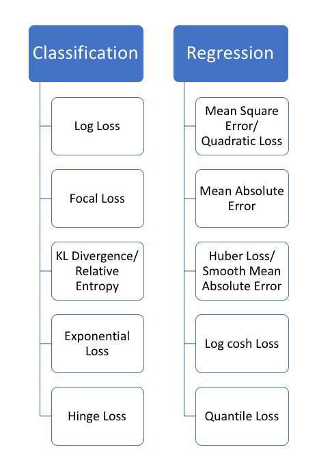
There are also other loss functions like Focal Loss(which we define in RetinaNet), SVM Loss(Hinge), KL Divergence, Huber Loss etc.

In next post, we will switch from vision to text, we will understand Bag of Model and Embeddings. Stay tuned!

Introduction to Object Detection

A long time ago in a galaxy far, far away….

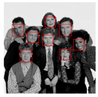
I-know-everything: My dear Padwan, unfortunately this will be our last post on vision. So, let’s make it count. Today we will see one of the most exciting applications of vision, Object Detection. There are literally thousands of application examples we can use object detection in for example, self-driving car detect whatever you see(through cameras) which includes traffic light, pedestrian, other cars, etc., counting particular objects for keeping track, surveillance(Not cool), or making a bot for following cats(Cool). Face Detection and Recognition is itself a bigger challenge with lots of exicting models like FaceNet, DeepFace, HyperFace etc and amazing datasets(Ask Google).

I-know-nothing: So, will it be like we pass a image and we get what objects are present in image along with their locations?

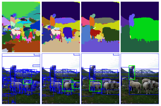
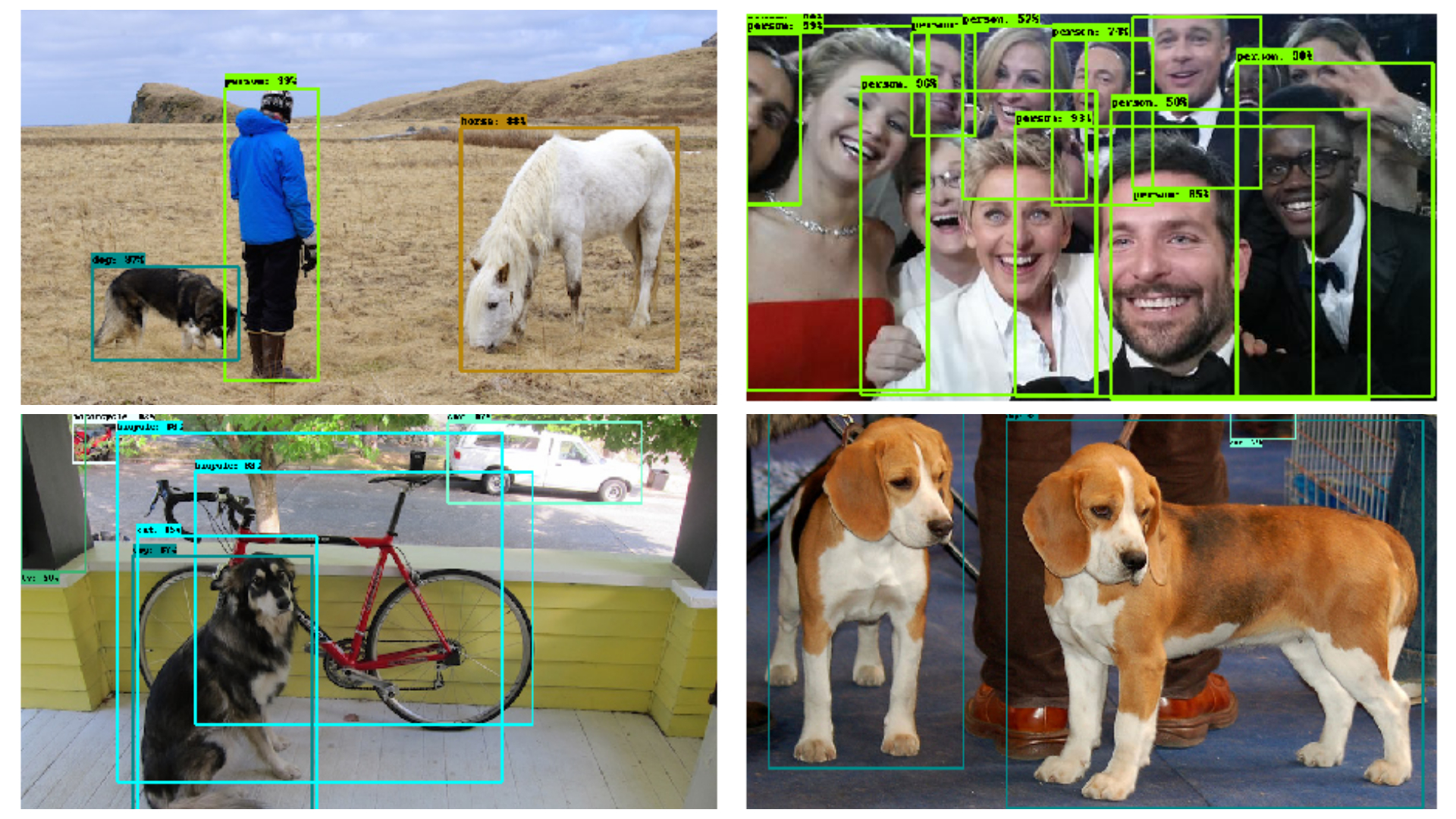
I-know-everything: Yes, exactly.(Always looking for end-to-end) And we can run these experiments real-time on video too. There is some subtle difference in different types of detections which I will let this puppies and cat explain it.

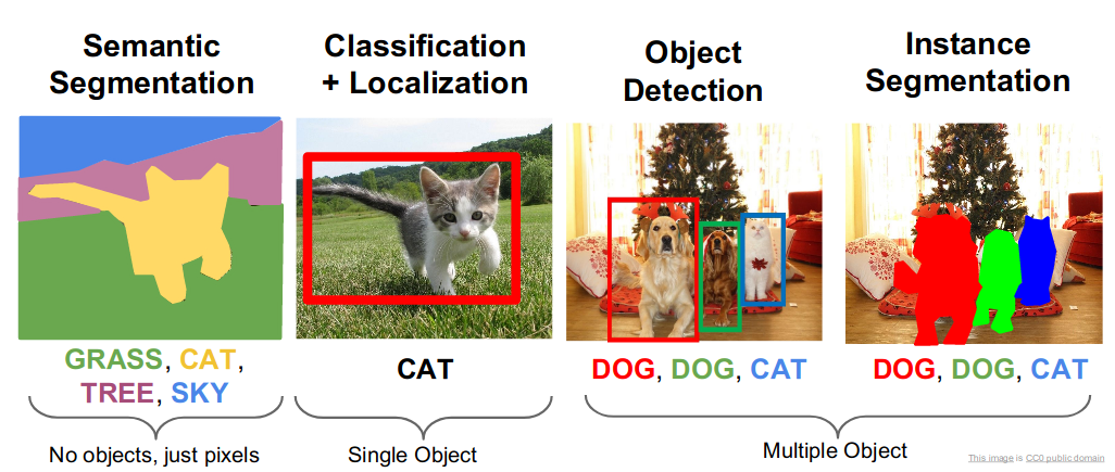
So, these are subtle differences in classification, localization, segmentation and instance segmentation. Here, the classification and localization task contains input single image and we are supposed to identify what class does that image belong to and where is it. But in object detection, this problem gets blown on a multiple scale. There can be any number of objects in image and each object will have different size in image, for given image we have to detect the category the object belong to and locate the object. This is what makes the challenge in detection very interesting.

Now, that you have understood what we are doing in object detection. Let’s look at some of the algorithms we can use to make such cool object detectors. I mean very cool.

Viola Jones Detector

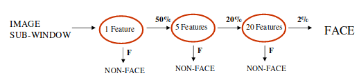
In early 2000s deep learning where in their infancy or deep learning where not everything, in this paper by Viola and Jones, they proposed a machine learning approach for visual object detection which is capable of processing images extremely rapidly and achieving high detection rates. The algorithm consisted of 3 important parts, integral images which consisted of calculating about 60,,000 image features, AdaBoost classifier, a boosting process which is collection of weak classifier and cascading where more complex classifier are cascaded in a chain. Intutivley, they created a chain of suppose 3 classifier, where each sub-window (field of view) classifies it as a “face or not a face”. Those sub-windows which are not intially rejected get passed on to next classifier and so no. If any classifier rejects sub-window, no further processing is involved. So, it was a degenerate decision classifier. This process allowed quick selection of faces and discarding backgrounds very quickly.

For example, in below classifier, 1 feature classifier achieves 100% detection rate with 50% false positive rate, 2 feature classifier with 100% detection rate and 40% false positive rate(20% cumulative) and 20 feature classifier achieve 100% detection rate with 10% false positive rate(2% cumulative).

Here are some results,

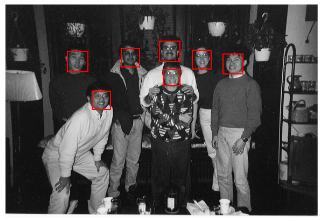
The real-time detector ran at 15 frames per second on a conventional 700 MHz Intel Pentium III.

For further, take a look at cool explaination by Dr. Mike Pound on Viola-Jones Algorithm on Computerphile.

OverFeat

One of the first deep learning approach using ConvNets was developed by LeCunn et al in architecture called Overfeat. They provide integrated approach to object detection, recognition and localization with a single ConvNet. As we have discussed before, in this algorithm there are two parts of network, classification and localization. The classification network(Overfeat architecture) is trained on Imagenet classifying object into one of 1000 categories. The classifier layers of classification network is replaced by regression network which predicts object bounding box at each spatial location and scale. In OverFeat, the region-wise features come from a sliding window of one aspect ratio over a scale pyramid. These features are used to simultaneously determine the location and category of objects. On the 200-class ILSVRC2013 detection dataset, OverFeat achieved mean average precision (mAP) of 24.3%. Let’s analyse the steps used in the algorithm:

Train a CNN model (similar to AlexNet) on the image classification task.
Replace the top classifier layers by a regression network and train it to predict object bounding boxes at each spatial location and scale. The regressor is class-specific, each generated for one image class.

The working of algorithm can be explained by an example of detecting bear shown below.

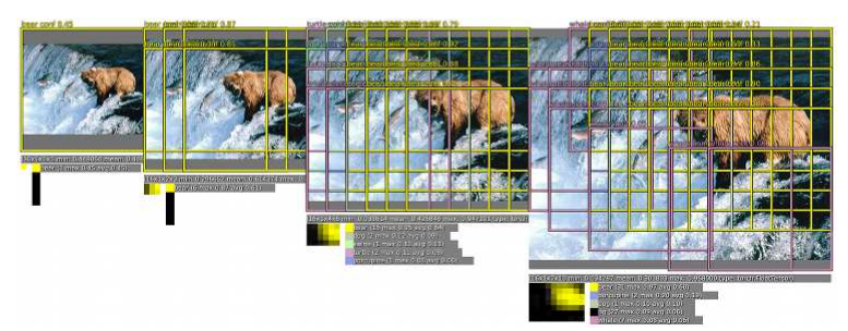
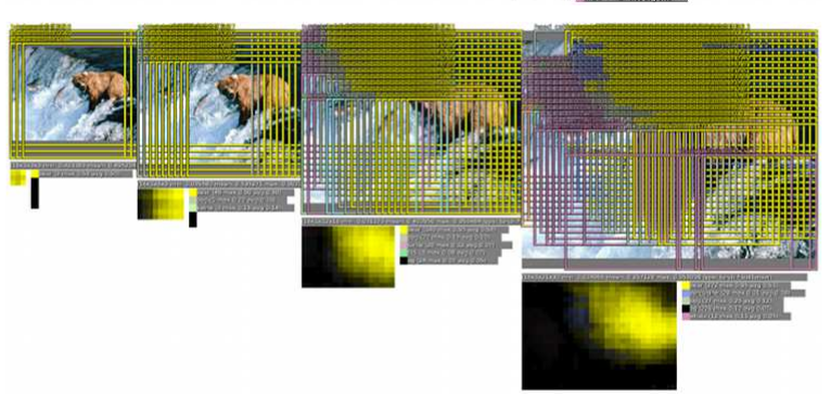
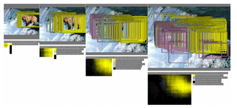
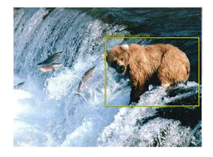
Using a sliding window approach method, which is effective in ConvNets as they share weights, the algorithm uses 6 different scales of input which are then presented to classifier to predict the class for each window for different resolutions as shown in top left and top right example. The regression then predicts the location scale of object with respect to each window as shown in bottom left and then these bounding boxes are merged and accumulated to a small number of objects as shown in bottom right. The various aspect ratios of the predicted bounding boxes shows that the network is able to cope with various object poses.

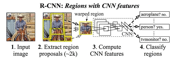
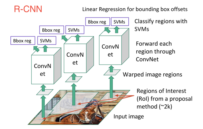
R-CNN

Introduction for using CNN for object detection gave rise to whole new networks and kept pushing the boundary of state-of-the-art detectors. Quickly after OverFeat, Grishick et al proposed a method where they used selective search to extract 2000 regions which they called “region proposals” (regions with high probability of containing objects). Hence the name, Regions with CNN features, R-CNN. They perform classification and regression on these 2000 region proposals. This result improved the previous result set by Overfeat on ILSVRC2013 detection dataset of 24.3% to 31.4%, an astounding 30% improvement. Let’s analyse the steps used in the algorithm:

Extract possible objects using a region proposal method (the most popular one being Selective Search) to some fixed size
Extract features from each region using a CNN
Classify each region with SVMs (using hinge loss)
Predict offset loss to correct the prediction values of location produced in region proposal stage (using least square l2 loss)

Selective Search

The sliding window based approach used a window (grid of size say 7 x 7) which scans across the whole image and send that to classifier to classify if it is an object or not a object. Then there are various aspect ratio to be considered inside an image as different object can have different sizes. So, classifying for each location becomes extremely slow. But what if somehow someone provided us with 2000 potentially object containing regions regardless of their relative sizes and then our only job is to classify and localize based on these 2000 region proposals.

Here come the role of selective search, which uses an hierarchical grouping algorithm, a greedy algorithm to iteratively group regions together. This selective search is used in R-CNN to generate 2000 Region Proposals which are then passed to classifier network.

The classifier network is AlexNet Network which acts as a feature extractor. For each proposal, a 4096-dimensional vector is computed which are then fed into SVM to classify the presence of the object within that candidate region proposal. This 4096-D vector also fed in a linear regressor to adapt the shapes of the bounding box for a region proposal and thus reduce localization errors.

Problems in R-CNN

It takes a lot of time to generate 2000 proposals for each image.(Can we propose a new algorithm to replace these fixed proposals?)
Real time object detection requires 47 seconds (not cool).
The selective search algorithm is a fixed algorithm. Therefore, no learning is happening at that stage. This could lead to the generation of bad candidate region proposals.(Can we propose a new algorithm which is not fixed?)
Training requires multiple stages of processing, where first ConvNet are finetuned to produce 4096-D vector. SVM uses these features to classify and in third stage bounding regressor are learned from feature vectors.(Could we somehow achieve classification and localization in parallel in one-shot?)

Training

Training routine consists of classifying object into N classes and also predicting predictions for bounding box containing object.

Typical training routine in all object detection algorithm consists of calculating Intersection Over Union (IOU), Non-max suppression (NMS) and loss. We will discuss about it below.

Intersection Over Union (IOU)

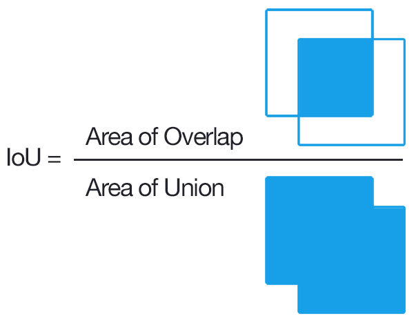
In the numerator we compute the area of overlap between the predicted bounding box and the ground-truth bounding box. The denominator is the area of union, or more simply, the area encompassed by both the predicted bounding box and the ground-truth bounding box. Dividing the area of overlap by the area of union yields our final score — the Intersection over Union.

Here is 3 different scenarios where orange is ground-truth and blue is predicted bounding box:

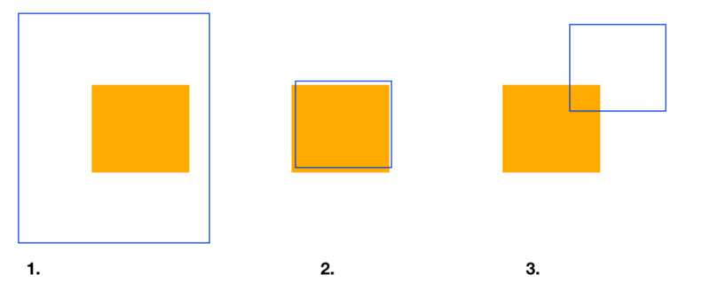
Poor IOU: Area of intersection is small compared to Area of Union which is greater, the ratio will be very low (Area of Intersection/Area of Union).
Near perfect IOU: Area of intersection and Area of Union are so close to each other. The ratio approaches 1.
Way off IOU: As area of intersection is very small compared to Area of Union.

As you can see, predicted bounding boxes that heavily overlap with the ground-truth bounding boxes have higher scores than those with less overlap.

An Intersection over Union score > 0.5 is normally considered a “good” prediction.

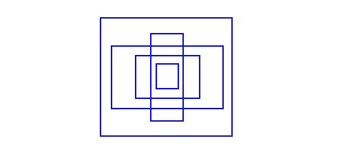
Anchor Boxes

It might make sense to predict the width and the height of the bounding box, but in practice, that leads to unstable gradients during training. Instead, most of the modern object detectors predict log-space transforms, or simply offsets to pre-defined default bounding boxes called anchors. Then, these transforms are applied to the anchor boxes to obtain the prediction.

Here is an example of 5 different anchor boxes,

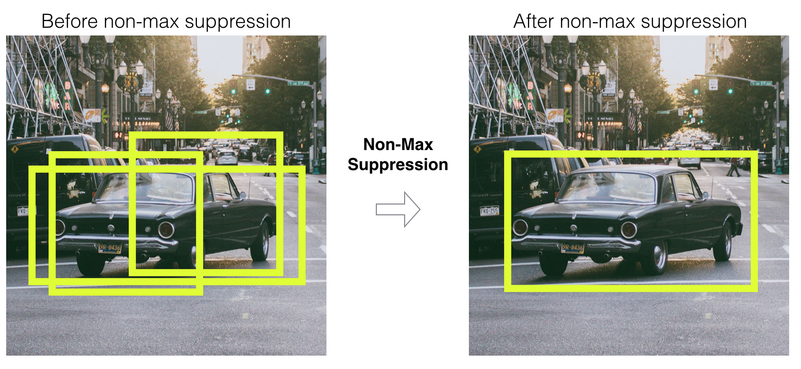
Non Max Suppresion(NMS)

Non-max suppression is a common algorithm used for cleaning up when multiple boxes are predicted for the same object. Here is how it works:

Discard all boxes with prediction confidence of object less or equal to 0.6
Pick the box with the largest prediction confidence output as a prediction
Discard any remaining box with IoU greater than or equal to 0.5

Mean Average Precision (mAP)

A common evaluation metric used in many object recognition and detection tasks is “mAP”, short for “mean average precision”. It is a number from 0 to 100; higher value is better. Here is how algorithm works:

Given that target objects are in different classes, we first compute AP (which is area under Precision-Recall curve) separately for each class, and then average over classes
A detection is a true positive if it has “intersection over union” (IoU) with a ground-truth box greater than some threshold (usually 0.5; if so, the metric is “mAP@0.5”)

Loss Functions

In general for all object detection algorithms, there are two main objective functions to minimize. The first one is classfication loss(\(\mathcal{L}_{cls}\)) which we have seen multiple times, but this classification loss is multi-class classification loss which translates to log-loss we defined above. The second loss function is regression loss(\(\mathcal{L}_{reg}\)) over predicted 4 values of bounding boxes which as we have defined above as combination of L1 loss and L2 loss also known as smooth L1 loss. Smooth L1-loss combines the advantages of L1-loss (steady gradients for large values of x) and L2-loss (less oscillations during updates when x is small).

\[\begin{aligned} \mathcal{L}_{smooth} = & \begin{cases} 0.5x^2 & |x| < 1\\ |x| - 0.5 & otherwise \end{cases} \end{aligned}\] \[\begin{aligned} \mathcal{L} = \mathcal{L}_{cls} + \mathcal{L}_{reg} \end{aligned}\]

Some algorithms minimize classification and regression together wherease some in two stages. But these two losses are present in all detectors.

Fast R-CNN

To overcome shortcomings of R-CNN, Grishick proposes Fast R-CNN which employs several innovations to improve training and testing speed while also increasing detection accuracy. Why not run the CNN just once per image and then find a way to share that computation across the ~2000 proposals? Let’s analyse the steps used in the algorithm:

An input is entire image and a set of object proposals
The network first processes the whole image with several convolutional (conv) and max pooling layers to produce a conv feature map
For each object proposal a region of interest (RoI) pooling layer extracts a fixed-length feature vector from the feature map
Each feature vector is fed into a sequence of fully connected (fc) layers that finally branch into two sibling output layers: one that produces softmax probability estimates over K object classes plus a catch-all background class and another layer that outputs four real-valued numbers for each of the K object classes. Each set of 4 values encodes refined bounding-box positions for one of the K classes

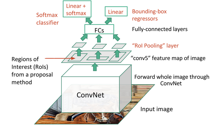
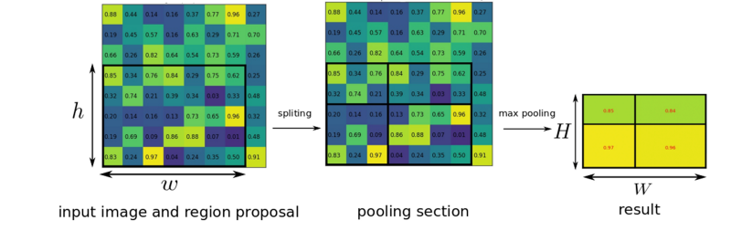
ROI Pooling

The RoI pooling layer uses max pooling to convert the features inside any valid region of interest into a small feature map with a fixed spatial extent of H×W (e.g. 7x7). In example below, with input ROI of 5×7, and output of 2×2, the area for each pooling area is 2×3 or 3×3 after rounding. Region of Interest Pooling allowed for sharing expensive computations and made the model much faster.

Advantages over R-CNN

Higher detection quality (mAP) than R-CNN
Training is single-stage, using a multi-task loss (no need of multi-stage as seen in RCNN)
Training can update all network layers (end-to-end)
Avoid feature caching as SVM is replaced by Softmax, no need to store feature vectors (softmax is better than SVM)

Problems in Fast R-CNN

Still requires region proposals from selective search algorithm
At runtime, the detection network processes images in 0.3s (excluding object proposal time)

Faster R-CNN

To overcome shortcomings of Fast R-CNN, Grishick(again!) et al proposes faster architecture than previous attempts, hence the name Faster R-CNN. The introduce a Region Proposal Network (RPN) that shares full-image convolutional features with the detection network, thus enabling nearly cost-free region proposals(finally). An RPN is a fully convolutional network that simultaneously predicts object bounds and objectness scores at each position. The RPN is trained end-to-end to generate high-quality region proposals, which are used by Fast R-CNN for detection. Let’s analyse the steps used in the algorithm:

Input the image to CNN to produce fixed feature map
Extracted feature map is sent to two different network: RPN and Fast R-CNN
RPN uses features to predict region proposals
Once we have these region proposals it’s just following Fast R-CNN algorithm where we want input, list of object proposals and input image

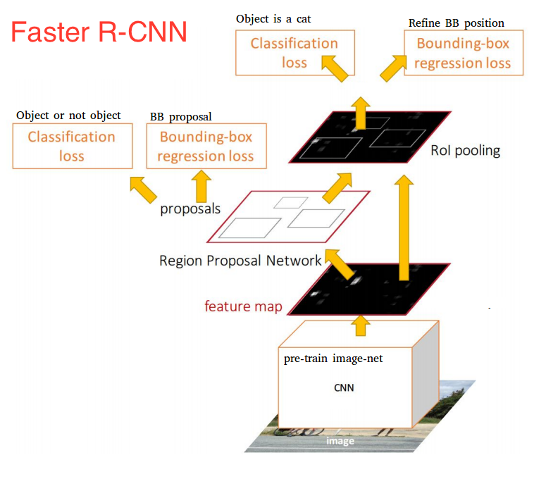
Region Propsal Network (RPN)

RPN were introduced to replace slow selective search which proposes region proposals with fast neural networks. Here is how RPN works:

First, the picture goes through conv layers and feature maps are extracted
Then a sliding window is used in RPN for each location over the feature map
For each location, k (k=9) anchor boxes (3 scales of 128, 256 and 512, and 3 aspect ratios of 1:1, 1:2, 2:1) are used for generating region proposals
A classification layer outputs 2k scores whether there is object or not for k boxes
A regression layer outputs 4k for the coordinates (box center coordinates, width and height) of k boxes
With a size of W×H feature map, there are WHk anchors in total

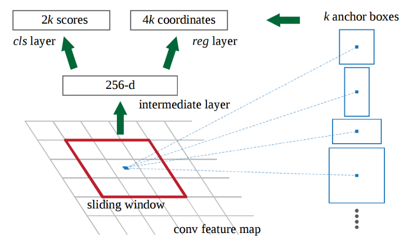
In Faster R-CNN, the “proposals” are dense sliding windows of 3 scales (128, 256, 512) and 3 aspect ratios (1:1, 1:2, 2:1).

Region of Interest Pooling (ROI)

After the RPN step, we have a bunch of object proposals with no class assigned to them. Our next problem to solve is how to take these bounding boxes and classify them into our desired categories.

The simplest approach would be to take each proposal, crop it, and then pass it through the pre-trained base network. Then, we can use the extracted features as input for a vanilla image classifier. The main problem is that running the computations for all the 2000 proposals is really inefficient and slow.

Faster R-CNN tries to solve, or at least mitigate, this problem by reusing the existing convolutional feature map. This is done by extracting fixed-sized feature maps for each proposal using region of interest pooling. Fixed size feature maps are needed for the R-CNN in order to classify them into a fixed number of classes.

Region-based CNN

Region-based convolutional neural network (R-CNN) is the final step in Faster R-CNN’s pipeline. After getting a convolutional feature map from the image, using it to get object proposals with the RPN and finally extracting features for each of those proposals (via RoI Pooling), we finally need to use these features for classification. R-CNN tries to mimic the final stages of classification CNNs where a fully-connected layer is used to output a score for each possible object class.

In Faster R-CNN, the R-CNN takes the feature map for each proposal, flattens it and uses two fully-connected layers of size 4096 with ReLU activation.

Then, it uses two different fully-connected layers for each of the different objects:

A fully-connected layer with N+1 units where N is the total number of classes and that extra one is for the background class.
A fully-connected layer with 4N units. We want to have a regression prediction

Jointly train for 4 losses RPN classify (object or not object), RPN regression box coordinates, final classification score(object classes), final box coordinates from Fast R-CNN.

Advantages over R-CNN and Fast R-CNN

Higher detection quality (mAP) than R-CNN and Fast R-CNN
At runtime, the detection network requires 200ms per image

Problems in Faster R-CNN

Two different networks(Can we combine everything in single network?)
Four loss functions to optimize (2 for RPN and 2 for Fast R-CNN)
Fully connected layers increase the parameters in network due to which inference time takes toll.(Can we get rid of dense layers?)

Results from pretrained model using tensorflow Object Detection API using Faster R-CNN with Inception pretrained model,

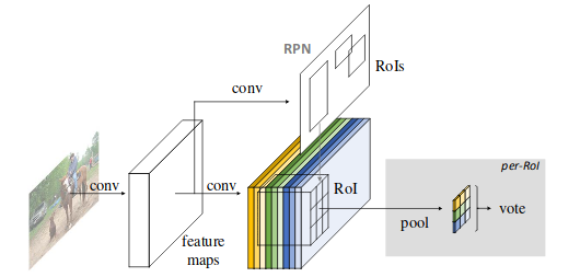
R-FCN

R-FCN uses region-based, fully convolutional networks based approach for object detection where almost all computation shared on the entire image. He et al propose a solution of using “position-sensitive score maps” which takes into account both translation invariance for image classification (wherever the object is in image) and translation variance for drawing boxes around the classified object i.e. object detection. Essentially, these score maps are convolutional feature maps that have been trained to recognize certain parts of each object. Let’s analyse the steps used in the algorithm:

Run a backbone network (here, ResNet-101) over input image
Add FCN to generate banks of \(k^2\) position-sensitive score maps for each category, i.e. \(k^2(C+1)\) output where \(k^2\) represents the number of relative positions to divide an object (e.g. \(3^2\) for a 3 by 3 grid) and C+1 representing the number of classes plus the background
Run a fully convolutional region proposal network (RPN) to generate regions of interest (RoI’s)
For each RoI, divide it into the same \(k^2\) “bins” or subregions as the score maps
For each bin, check the score bank to see if that bin matches the corresponding position of some object. This process is repeated for each class
Once each of the \(k^2\) bins has an “object match” value for each class, average the bins to get a single score per class
Classify the RoI with a softmax over the remaining (C+1) dimensional vector

In short, Region Proposal Network (RPN), which is a fully convolutional architecture is used to extract candidate regions. Given the proposal regions (RoIs), the R-FCN architecture is designed to classify the RoIs into object categories and background.

Position-sensitive score maps and Position-sensitive ROI pooling

The last convolutional layer of produces a bank of \(k^2\) position-sensitive score maps for each category, and thus has a \(k^2(C+1)\) -channel output layer with C object categories (+1 for background). The bank of \(k^2\) score maps correspond to a k x k spatial grid describing relative positions. For example, with k x k = 3 x 3, the 9 score maps encode the cases of {top-left, top-center, top-right, …, bottom-right} of an object category.

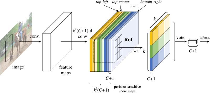
When ROI pooling, (C+1) feature maps with size of \(k^2\) are produced, i.e. \(k^2(C+1)\). The pooling is done in the sense that they are pooled with the same area and the same color in the figure. Average voting is performed to generate (C+1) 1d-vector. And finally softmax is performed on the vector.

Consider for example following example of R-FCN detecting a baby,

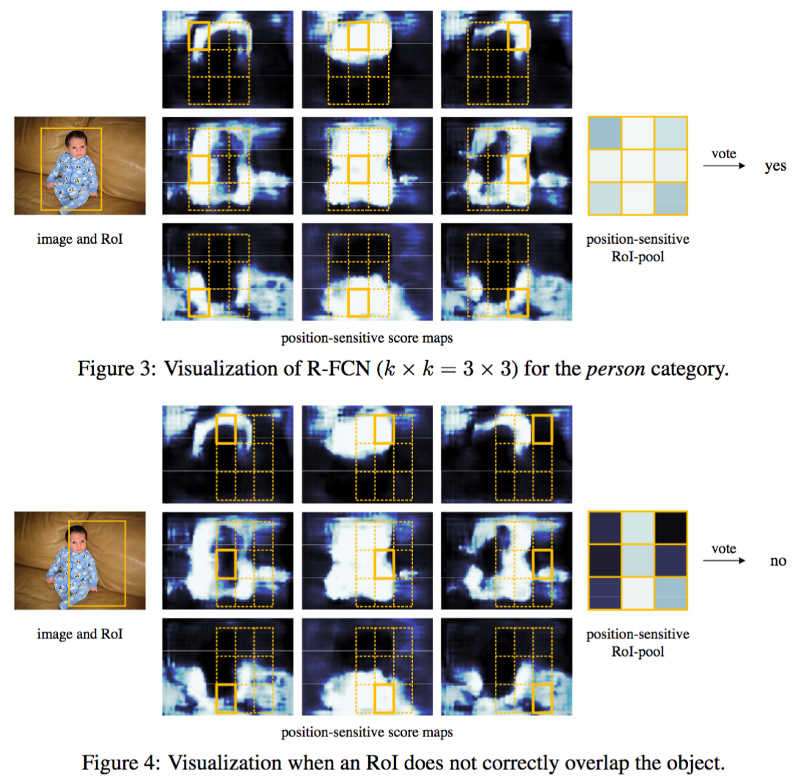
As Joyce Xu explains above example as,

Simply put, R-FCN considers each region proposal, divides it up into sub-regions, and iterates over the sub-regions asking: “does this look like the top-left of a baby?”, “does this look like the top-center of a baby?” “does this look like the top-right of a baby?”, etc. It repeats this for all possible classes. If enough of the sub-regions say “yes, I match up with that part of a baby!”, the RoI gets classified as a baby after a softmax over all the classes.

Advantages over Faster R-CNN

The result is achieved at a test-time speed of 170ms per image. Faster than Faster R-CNN.
Comparable detection quality (mAP) to Faster R-CNN

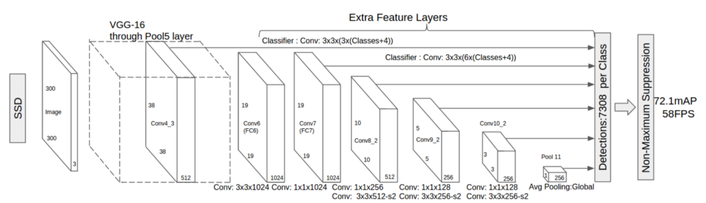
SSD

SSD is simple relative to previous methods that require object proposals because it completely eliminates proposal generation (wooh) and subsequent pixel or feature resampling stages and encapsulates all computation in a single network(yay). Hence, the name single shot detector (SSD). One model to solve them all. Simply remarkable. Let’s analyse the steps used in the algorithm:

Pass the image through a series of convolutional layers, yielding several sets of feature maps at different scales (e.g. 10x10, then 6x6, then 3x3, etc.)
For each location in each of these feature maps, use a 3x3 convolutional filter to evaluate a small set of default bounding boxes. These default bounding boxes are essentially equivalent to Faster R-CNN’s anchor boxes
For each box, simultaneously predict a) the bounding box offset and b) the class probabilities
During training, match the ground truth box with these predicted boxes based on IoU. The best predicted box will be labeled a “positive,” along with all other boxes that have an IoU with the truth >0.5

To put it simply, SSD approach is based on a feed-forward convolutional network that produces a fixed-size collection of bounding boxes and scores for the presence of object class instances in those boxes, followed by a non-maximum suppression step to produce the final detections.

Choosing scales and aspect ratios for default boxes

There are “extra feature layers” as seen in above architecture at the end that scale down in size. These varying-size feature maps help capture objects of different sizes, where each feature map is associated with a set of default bouding boxes. At each feature map cell, network predict the offsets relative to the default box shapes in the cell, as well as the per-class scores that indicate the presence of a class instance in each of those boxes. Specifically, for each box out of k at a given location, network computes c class scores and the 4 offsets relative to the original default box shape. This results in a total of (c + 4)k filters that are applied around each location in the feature map, yielding (c + 4)kmn outputs for a m × n feature map. Default boxes are similar to the anchor boxes used in Faster R-CNN only they are applied to several feature maps of different resolutions.

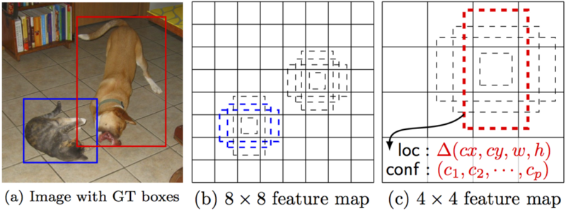
Consider above example where, SSD evaluates a small set (e.g. 4) of default boxes of different aspect ratios at each location in several feature maps with different scales (e.g. 8 x 8 and 4 x 4 in middle and right images). For each default box, SSD predict both the shape offsets and the confidences for all object categories belonging to C categories. At training time, SSD first match these default boxes (middle and right) to the ground truth boxes (left image). For example, SSD have matched two default boxes with the cat and one with the dog, which are treated as positives and the rest as negatives.

Challenges in Training

Hard Negative Mining

After matching, wherein authors match default boxes to any ground truth with jaccard overlap higher than a threshold (0.5), most of the default boxes are negatives, especially when the number of possible default boxes is large. This introduces a significant imbalance between the positive and negative training examples. Instead of using all the negative examples as seen from above example which can be a lot in proportion to positive, authors sort them using the highest confidence loss for each default box and pick the top ones so that the ratio between the negatives and positives is at most 3:1.

Data Augmentation

Data augmentation is crucial. To make the model more robust to various input object sizes and shapes, each training image is randomly sampled by one of the following options: use the entire original input image or sample a patch so that the minimum jaccard overlap with the objects is 0.1, 0.3, 0.5, 0.7, or 0.9. or randomly sample a patch. The size of each sampled patch is [0.1, 1] of the original image size, and the aspect ratio is between \(\frac{1}{2}\) and 2. An improvement of 8.8% mAP is observed due to this strategy.

The model loss is a weighted sum between localization loss (e.g. Smooth L1) and confidence loss (e.g. Softmax).

Advantages over Faster R-CNN

The real-time detection speed is just astounding and way way faster (59 FPS with mAP 74.3% on VOC2007 test, vs. Faster R-CNN 7 FPS)
Better detection quality (mAP) than any before
Everything is done in single shot. Single network to solve them all (Finally)

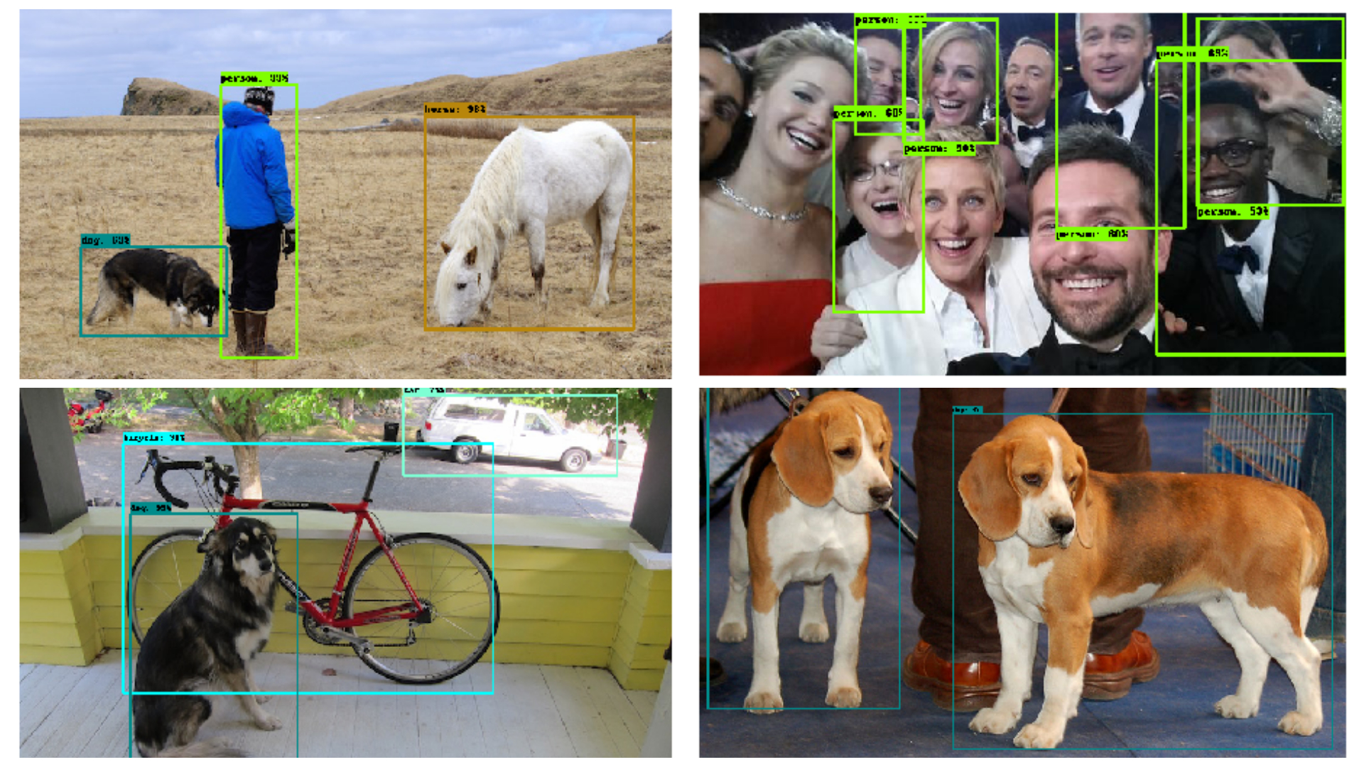
Here are some results using SSD and Inception as backbone architecture,

YOLO

You Only Live Once. No, it’s not that. YOLO is You Only Look Once. So, cool. Wonder how would have they come with such cool acroynm. Over the period of 3 years, 3 different versions of same algorithm with slight variations were proposed. Let’s have a look at them one by one.

YOLOv1

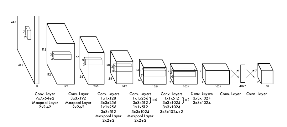
YOLOv1 was the first algorithm to unite detection and localization in single network. Everything achieved in end-to-end fashion. Input to model, model does something and comes with predicted output (both class probability and location of object). Ross Girshick (he’s back!) et al proposes a single convolutional network simultaneously predicts multiple bounding boxes and class probabilities for those boxes. YOLOv1 trains on full images and directly optimizes detection performance. Let’s analyse the steps used in the algorithm:

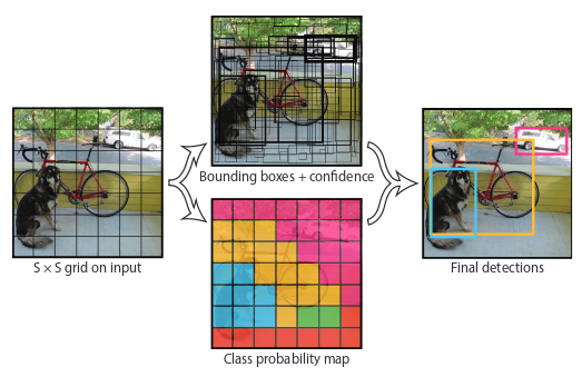
Input image passed to CNN network is divided into S x S grid (S = 7). If the center of an object falls into a grid cell, that grid cell is responsible for detecting that object.
Each grid cell predicts B bounding boxes and confidence scores for those boxes. If no object exists in that cell, the confidence scores should be zero.
Each bounding box consists of 5 predictions: x, y, w, h and confidence. The (x, y) coordinates represent the center of the box relative to the bounds of the grid cell. The width and height are predicted relative to the whole image. The confidence prediction represents the IOU between the predicted box and any ground truth box.
Each grid cell also predicts C conditional class probabilities, Pr(\(Class_{i}\) | Object). These probabilities are conditioned on the grid cell containing an object.

To put it simply, the model takes an image as input. It divides it into an SxS grid. Each cell of this grid predicts B bounding boxes with a confidence score. This confidence is simply the probability to detect the object multiply by the IOU between the predicted and the ground truth boxes.

Here is an example of detecting 3 objects, a dog, car and bicycle.

Problems in YOLOv1

Struggles with small objects that appear in groups, such as flocks of birds
Struggles to generalize to objects in new or unusual aspect ratios or configurations
Low detection (mAP) compared to previous region proposals methods

Advantages over Faster R-CNN

The real-time detection speed was extremely faster (before SSD came) (45 fps and fast yolo v1 achieves 155 fps really?)
Single network that does not require any region proposals or selective search

YOLOv2

Redmond et al proposed YOLOv2 which the second version of the YOLO with the objective of more accurate detector that is still fast. Here are some things that are have improved when compared to previous YOLOv1.

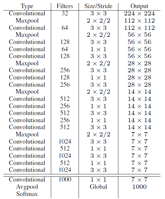
New CNN architecture: Darknet (Joining the dark side, are we?)

Batch Normalization: By adding batch normalization on all of the convolutional layers in YOLO, more than 2% improvement in mAP
High Resolution Classifier: In YOLOv2, authors first fine tune the classification network at the full 448 × 448 resolution for 10 epochs on ImageNet. This gives the network time to adjust its filters to work better on higher resolution input. Then fine tune the resulting network on detection. This high resolution classification network gives us an increase of almost 4% mAP. This enables the detection of potentially smaller objects one of the problems in YOLOv1.
Anchor Boxes: This got rid of one of critical problem in YOLOv1 about the ability to generalize to objects in new aspect ratios. Fully connected layers from YOLOv1 are removed and the new model uses anchor boxes to predict bounding boxes. Model uses 5 anchor boxes and predicts class and objectness for every anchor box. Using anchor boxes we get a small decrease in accuracy from 69.5 mAP to 69.2 mAP but recall increases from 81% to 88%.
Dimension Clustering: In YOLOv1, the dimension of boxes were prechosen. Instead of choosing anchor boxes dimensions by hand, authors propose using k-means clustering on the training set bounding boxes to automatically find good anchor boxes.
Direct Location Prediction: Instead of predicting offsets same approach of YOLO for predict location coordinates relative to the location of the grid cell is used and logistic activation bounds the ground truth to fall between 0 and 1. Using dimension clusters along with directly predicting the bounding box center location improves YOLO by almost 5% over the version with anchor boxes.
Fine-Grained Features: For detecting large objects, YOLOv2 outputs a predict feature map of 13 x 13. To detect small objects well, the 26×26×512 feature maps from earlier layer is mapped into 13×13×2048 feature map, then concatenated with the original 13×13 feature maps for detection. This leads to 1% performance increase.
Multi-Scale Training: YOLOv2 uses multiple of 32 new image dimension size every 10 batch, as network is downsampled by a factor of 32 from set of {320, 352, … 608}. This regime forces the network to learn to predict well across a variety of input dimensions. This means the same network can predict detections at different resolutions. The network runs faster at smaller sizes so YOLOv2 offers an easy tradeoff between speed and accuracy.

Problems in YOLOv2

Can we make it faster and more accurate?

Advantages over YOLOv1

The real-time detection speed was faster than YOLOv1
Way better detection quality (mAP) than YOLOv1 and SSD300 but slightly behind SSD512

YOLOv3

IMO, this is one of the coolest technical paper ever written. We need more of these. Bunch of cool upgrades to YOLOv2, YOLOv3 is a little bigger than last time but more accurate and fast. Here are some upgrades:

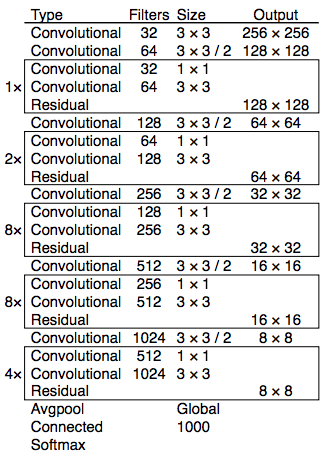
New CNN architecutre with 53 layers, or popularly known among dark side as Darknet-53.

Replace softmax with independent logistic classifiers. Using a softmax imposes the assumption that each box has exactly one class which is often not the case. A multilabel approach better models the data.
YOLOv3 predicts boxes at 3 different scales and extracts features from those scales using a similar concept to feature pyramid networks. Model predicts a 3-d tensor encoding bounding box, objectness, and class predictions. For e.g. N x N x (3 * (4 + 1 + C)) for the 4 bounding box offsets, 1 objectness prediction, and C class predictions.
Choose 9 clusters and 3 scales arbitrarily and then divide up the clusters evenly across scales. For e.g. (10 x 13), (16 x 30), (33 x 23), (30 x 61), (62 x 45), (59 x 119), (116 x 90), (156 x 198), (373 x 326).

Advantages over all before architectures

YOLOv3 is much better than SSD variants and comparable to state-of-the-art model (not, RetinaNet though which takes 3.8x longer to process an image) and very very fast

Here are some results using YOLOv3,

RetinaNet

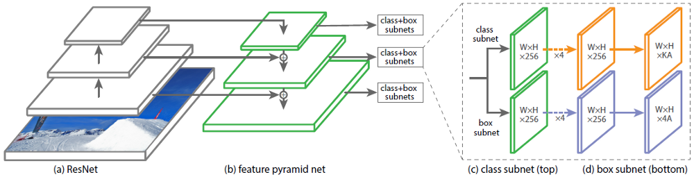
Girshick(yup again!) et al propose a new loss function Focal loss to deal with the foreground-background class imbalance posed in one-stage detectors. Okay, wait let me explain what do I mean by it exactly. From above so many architecture, there is one clear distinction that some architecture are one-shot detectors and others are two-shot detectors. In two-shot detectors, Region Proposal Networks provides potential regions to look at and second-stage classify so there is a good balance between foreground-background classes and but in one-shot network as we see in case of SSD, after matching there are lots of negatives and so less positives. They deal with a technique called Hard Negative Mining. So, the two-shot detectors provide greater accuracy than one-shot detector. Authors assert that after replacing standard cross entropy criterion with focal loss, they are able to match the speed of previous one-stage detectors while surpassing the accuracy of all existing state-of-the-art two-stage detectors. RetinaNet uses ResNet-101-FPN as backbone architecture and two-task specific subnetworks(classification and localization). It is combination of anchors used in all previous architectures and feature pyramids used in SSD.

Focal Loss

The loss function is a dynamically scaled cross entropy loss, where the scaling factor decays to zero as confidence in the correct class increases. Intuitively, this scaling factor can automatically down-weight the contribution of easy examples during training and rapidly focus the model on hard examples. Easy example, ahh? These are the examples where it is very easy to classify the given region as background. The class imbalance causes two problems: (1) training is inefficient as most locations are easy negatives that contribute no useful learning signal; (2) the easy negatives can overwhelm training and lead to degenerate models.

\[\begin{aligned} \mathcal{L} = -\alpha_{t}(1-\mathbf{p}_{t})^\gamma\log_{}{\mathbf{p}_{t}} \end{aligned}\]

Here \(\alpha_{t}\) weight assigned to rare class and \(\gamma\) focuses more on hard examples. In practice, \(\alpha\) = 0.25 and \(\gamma\) = 2 works best.

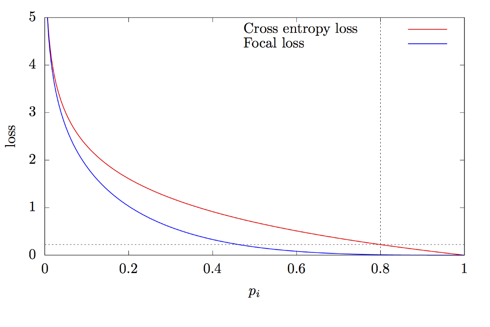
Let’s make this concrete with an example,

Scenario 1: Easy classified example

Suppose we have easy classified foreground object and background object with p=0.9 and p=0.1 respectively where p is probability of containig an object. If we calculate cross entropy and focal loss for each object (\(\alpha\) = 0.25 and \(\gamma\) = 2), we get

CE(foreground) = -log(0.9) = 0.1053

CE(background) = -log((1-0.1)) = 0.1053

FL(foreground) = -1 x 0.25 x \((1–0.9)^2\) log(0.9) = 0.00026

FL(background) = -1 x 0.25 x \((1–(1–0.1))^2\) log(1–0.1) = 0.00026

Scenario 2: Misclassified example

Suppose we have misclassified foreground object and misclassified background object with p=0.9 and p=0.1 respectively where p is probability of containig an object. If we calculate cross entropy and focal loss for each object (\(\alpha\) = 0.25 and \(\gamma\) = 2), we get

CE(foreground) = -log(0.1) = 2.3025

CE(background) = -log((1-0.9)) = 2.3025

FL(foreground) = -1 x 0.25 x \((1–0.1)^2\) log(0.1) = 0.4667

FL(background) = -1 x 0.25 x \((1–(1–0.9))^2\) log(1–0.9) = 0.4667

Scenario 3: Very easy classified example

Suppose we have very easy classified foreground object and background object with p=0.99 and p=0.01 respectively where p is probability of containig an object. If we calculate cross entropy and focal loss for each object (\(\alpha\) = 0.25 and \(\gamma\) = 2), we get

CE(foreground) = -log(0.99) = 0.004

CE(background) = -log((1-0.01)) = 0.004

FL(foreground) = -1 x 0.25 x \((1–0.99)^2\) log(0.99) = 2.5 x 1e-7

FL(background) = -1 x 0.25 x \((1–(1–0.01))^2\) log(1–0.01) = 2.5 x 1e-7

Scenario-1: 0.1/0.00026 = 384x smaller number

Scenario-2: 2.3/0.4667 = 5x smaller number

Scenario-3: 0.004/0.00000025 = 16,000x smaller number.

These three scenarios clearly show that Focal loss add very less weight to well classified examples and large weight to misclassified or hard classified examples.

Backbones

This base is responsible for creating a feature map that is embedded with salient information about the image. The accuracy for the object detector is highly related to how well the convolutional base(backbones) can capture meaningful information about the image. The base takes the image through a series of convolutions that make the image smaller and deeper. This process allows the network to make sense of the various shapes in the image. Many of the detection algorithms use of the following backbone architecture depending on trade-off in inference speed and accuracy, space vs latency. These are called backbone architecture which forms a base for detection algorithms upon which we add subnetworks for classifications and regression tasks.

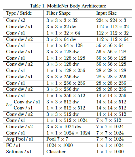
MobileNet

As the name suggests, this network is more suitable for low power appliances like mobile and embedded applications. MobileNets are light weight because they use depthwise separable convolutions.

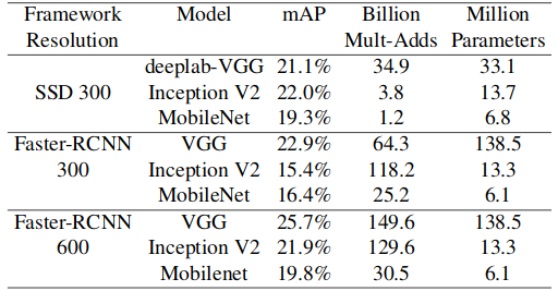
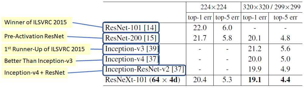
Here is a comparison of different backbones versus MobileNet,

ResNeXt

ResNext draws inspiration from lot of architecture. VGG-nets and ResNets show imple yet effective strategy of constructing very deep network by stacking building blocks of same shape. The Inception models adopt split-transform-merge strategy. ResNext combines these two strategies. It’s simple design compared to ResNet architecture and accurate.

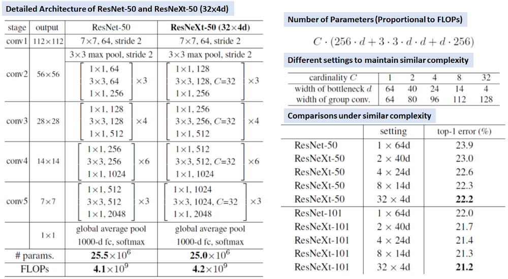
Here is a comparison of different architecture versus MobileNet,

Feature Pyramid Networks

Feature pyramids are a basic component in recognition systems for detecting objects at different scales. But are avoided as they are compute and memory intensive. FPN construct feature pyramids with lateral connections is developed for building high-level semantic feature maps at all scales.

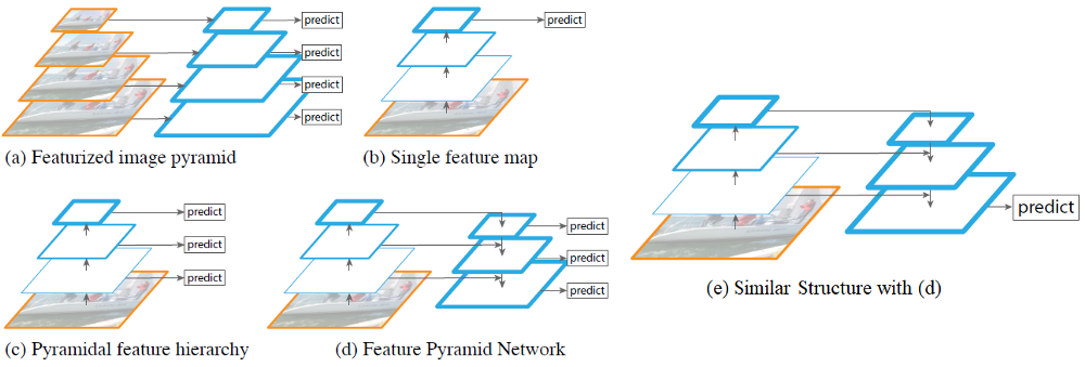
We have seen different architecture from above in various detector models. (b) is used in YOLO, (c) is used in SSD, (d) is FPN where it combines low-resolution, semantically strong features with high-resolution, semantically weak features via a top-down pathway and lateral connections.

The other many othet backbones include ResNet, VGG, Inception, InceptionResNet etc.

Here is a table of comparison to summarize the results on VOC 2007 test dataset of all detectors. Table borrowed from this paper.

Methods	Trained on	mAP(%)	Test time(sec/img)	FPS
R-CNN	07	66.0	32.84	0.03
Fast R-CNN	07 + 12	66.9	1.72	0.6
Faster R-CNN(Resnet)	07 + 12	83.8	2.24	0.4
R-FCN	07 + 12 + coco	83.6	0.17	5.9
SSD300	07 + 12	74.3	0.02	46
SSD512	07 + 12	76.8	0.05	19
YOLOv1	07 + 12	63.4	0.02	45
YOLOv2	07 + 12	78.6	0.03	40

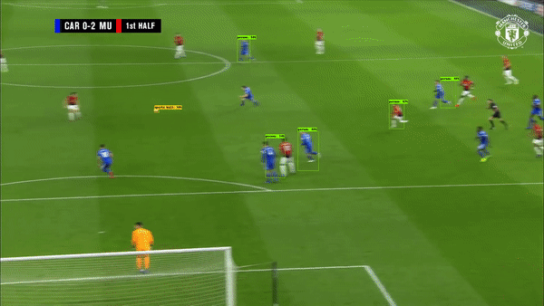
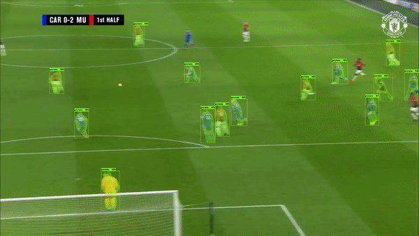
Here is some result from using object detection on video.

Recap

Here is a quick recap, so we saw there are broadly two types, two-stage detectors and one-stage detectors. In two-stage detector, region proposals are given by some fancy selective search algorithms which reduces the overhead of searching all over the image for finding objects, these are then passed to classification and regression subnetworks which do their job of classifying and localizing different objects present in the image. This can be seen in all R-* detectors, RCNN, FastRCNN, Faster-RCNN and RFCN. Next, we looked at one-stage detectors, these type of detectors don’t require any input of region proposals, just give them image, they will output classes of object and their locations. This can be seen in family of algorithms like SSD, YOLO(v1, v2, v3). But then we learned that one-shot detectors even though they provide excellent real-time speed(fps) but they are not as accurate in detection as two-stage detectors. Then came the role of RetinaNet, which proposes new loss function, focal loss, which handles the trade-off between accuracy and latency real smooth. Having looked at family of object detectors, we looked at some of the driving architectures behind these detectors which can be ResNet, VGG or MobileNets, etc depending on how accurate or how fast is the requirement. This was a fascinating challenge but no detection algorithm can match detection going on in our brain.

This completes our journey in Object Detection Land.

This only explains Mystery of Object Detection, then we have Semantic Segementation and Instance Segmentation. One notable architecture from both are U-Net and Mask R-CNN respectively. Mask R-CNN results are so cool!

Here is a glimpse of result from Mask R-CNN which is instance segmentation algorithm.