Tabular Solution Methods

All the codes implemented in Jupyter notebook DP, MC and TD.

All codes can be run on Google Colab (link provided in notebook).

Feel free to jump anywhere,

Terminologies
Tabular Solution Methods
Further Reading
Footnotes and Credits

Terminologies

Before diving deep into Tabular RL methods used to solve RL problems, we will visit some terminologies that will be mentioned frequently in our discussion of various algorithms.

Markov Process

In Markov processes, the states captures all relevant information from the past agent–environment interaction. These states are said to have Markov property. The states with Markov property are memoryless. For e.g we can predict the next move on chess board given any configuration of the board i.e. all that matter to predict the next move is the current state. It doesn’t matter how we got there. The current state is a sufficient statistic of the future.

The future is independent of the past given the present.

\[\begin{aligned} P(S_{t} \vert S_{1}, S_{2}, ..., S_{t-1}) = P(S_{t} \vert S_{t-1}) \end{aligned}\]

Markov Process(or Markov Chain) is a tuple (\(\mathcal{S}\), \(\mathcal{P}\)),

\(\mathcal{S}\) is a (finite) set of states
\(\mathcal{P}\) is a state transition probability matrix, \(\mathcal{P}_{ss^{'}}\) = \(\mathbb{P}[S_{t+1} = s^{'} \vert S_{t} = s]\)

Markov Reward Process

A Markov reward process is a Markov chain with values. In Markov reward processes, each transition is associated with a reward. The agent-environment interaction can be episodic i.e. broken into episodes, terminating after ending up in a terminal state or continuous in which the interaction does not naturally break into episodes but continues without limit. That is why we, introduce a discounted delayed reward. If \(\gamma\) = 0, we get a myopic agent concerned only with maximising immediate rewards and \(\gamma\) = 1, we get a far-sighted agent which takes future rewards into account more strongly.

Markov Reward Process is a tuple (\(\mathcal{S}\), \(\mathcal{P}\), \(\mathcal{R}\), \(\gamma\)),

\(\mathcal{S}\) is a (finite) set of states
\(\mathcal{P}\) is a state transition probability matrix, \(\mathcal{P}_{ss^{'}}\) = \(\mathbb{P}[S_{t+1} = s^{'} \vert S_{t} = s]\)
\(\mathcal{R}\) is a reward function, \(\mathcal{R}_{s}\) = \(\mathbb{E}[\mathcal{R}_{t+1} \vert S_{t} = s]\)
\(\gamma\) is a discount factor, \(\gamma \in\) [0, 1]

Markov Decision Process

A Markov decision process (MDP) is a Markov reward process with decisions. Markov decision process(MDP) is used to describe an environment in reinforcement learning. In MDPs, we are concerned with selecting different action associated with every state. The environment responds with a new state and reward for choosing a particular action when in a given particular state. Almost all RL problems can be formalised as MDPs.

Markov Decision Process is a tuple (\(\mathcal{S}\), \(\mathcal{A}\), \(\mathcal{P}\), \(\mathcal{R}\), \(\gamma\)),

\(\mathcal{S}\) is a (finite) set of states
\(\mathcal{A}\) is a (finite) set of actions
\(\mathcal{P}\) is a state transition probability matrix, \(\mathcal{P}^{a}_{ss^{'}}\) = \(\mathbb{P}[S_{t+1} = s^{'} \vert S_{t} = s, A_{t} = a]\)
\(\mathcal{R}\) is a reward function, \(\mathcal{R}_{s}\) = \(\mathbb{E}[\mathcal{R}^{a}_{t+1} \vert S_{t} = s, A_{t} = a]\)
\(\gamma\) is a discount factor, \(\gamma \in\) [0, 1]

Bellman Expectation Equation

A Bellman equations, named after Richard E. Bellman are the most fundamental equations in RL to solve the MDPs. Bellman equation deals with two types of problem, prediction and control solved using Bellman expectation equation and Bellman optimality equation. Bellman expectation equation deal with evaluating given policy while Bellman optimality are tasked with finding optimal policy and thus solving the MDP. We use bellman equation to show how current state is related to successive state for both value functions. We can apply this recursive equation for each sequence in each episode of an episodic task.

Returns

In RL, we seek to maximise the expected return where the return \(G_{t}\) is the total discounted reward from time-step \(t\).

For episodic tasks, \(G_{t} = R_{t+1} + R_{t+2} ... + R_{T}\), where T is the terminal state.

For continuous tasks, \(G_{t} = R_{t+1} + \gamma * R_{t+2} ... + \gamma^{2} * R_{t+3} = \sum_{k=0}^{\infty} \gamma^{k} R_{t+k+1}\), where \(\gamma\) is the discount rate.

The recursive equation of relating return at current time step \(t\) to next time step \(t+1\) is given by,

\[\begin{aligned} G_{t} = R_{t+1} + \gamma * G_{t+1} \end{aligned}\]

Value Functions

Almost all reinforcement learning algorithms involve estimating value functions. Value functions determine how good is it to be in a particular state (state-value function) or how good is to take a particular action in given state (action-value function). The state-value function and action-value function are related by the following equation,

\[\begin{aligned} v_{\pi}(s) &= \sum_{a \in A}\pi(a \vert s)q_{\pi}(s, a) \end{aligned}\]

State-value function

The state-value function of an MDP is expected return starting from state \(s\), and then following policy \(\pi\).

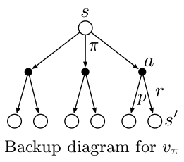
\[\begin{aligned} v_{\pi}(s) &= \mathbb{E}_{\pi}[G_{t} \vert S_{t} = s]\\ &= \mathbb{E}_{\pi}[R_{t+1} + \gamma v_{\pi}(S_{t+1}) \vert S_{t} = s]\\ &= \sum_{a \in \mathcal{A}}\pi(a \vert s)[\mathcal{R}_{s}^{a} + \gamma \sum_{s^{'} \in \mathcal{S}}\mathcal{P}_{ss^{'}}^{a}v_{\pi}(s^{'})]\\ \end{aligned}\]

This equation is Bellman equation for \(v_{\pi}\). When in state \(s\), an agent takes an action \(a\) based on its policy \(\pi\). The environment responds with one of several next states \(s^{'}\) along with immediate reward \(r\).

Bellman equation averages over all the possibilities, weighting each by its probability of occurring. It expresses a relationship between the value of a state and the values of its successor states.

Action-value function

The action-value function of an MDP is expected return starting from state \(s\), taking action \(a\) and then following policy \(\pi\).

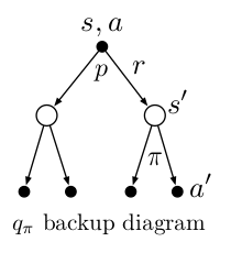
\[\begin{aligned} q_{\pi}(s, a) &= \mathbb{E}_{\pi}[G_{t} \vert S_{t} = s, A_{t} = a]\\ &= \mathbb{E}_{\pi}[R_{t+1} + \gamma q_{\pi}(S_{t+1}, A_{t+1}) \vert S_{t} = s, A_{t} = a]\\ &= \mathcal{R}_{s}^{a} + \gamma \sum_{s^{'} \in \mathcal{S}}\mathcal{P}_{ss^{'}}^{a}\sum_{a^{'} \in \mathcal{A}}\pi(a^{'} \vert s{'})q_{\pi}(s^{'}, a^{'}) \end{aligned}\]

This equation is Bellman equation for \(q_{\pi}\). When in state \(s\) and taking an action \(a\) based on its policy \(\pi\). The environment responds by sending agent to one of the several next states \(s^{'}\) that an agent can end up in, along with immediate reward \(r\).

Bellman Optimality Equation

Bellman Optimality Equation is based on the principle of optimality where an optimal policy has the property that whatever the initial state and initial decision are, the remaining decision must constitute an optimal policy with regard to the state resulting from the fist decision. Using bellman optimality equations, we find optimal way to solve any given MDP environment.

Optimal State-value Function

The optimal state-value function \(v_{*}(s)\) is the maximum state-value function over all policies.

\[\begin{aligned} v_{*}(s) &= max_{\pi}v_{\pi}(s)\\ &= max_{a \in \mathcal{A}}[\mathcal{R}_{s}^{a} + \gamma \sum_{s^{'} \in \mathcal{S}}\mathcal{P}_{ss^{'}}^{a}v_{\pi}(s^{'})] \end{aligned}\]

Optimal Action-value Function

The optimal action-value function \(q_{*}(s, a)\) is the maximum action-value function over all policies.

\[\begin{aligned} q_{*}(s, a) &= max_{\pi}q_{\pi}(s, a)\\ &= \mathcal{R}_{s}^{a} + \gamma \sum_{s^{'} \in \mathcal{S}}\mathcal{P}_{ss^{'}}^{a}max_{a^{'} \in \mathcal{A}}q_{\pi}(s^{'}, a^{'}) \end{aligned}\]

Optimal Policy

A policy is defined to be better than or equal to a policy \(\pi^{'}\) if its expected return is greater than or equal to than of \(\pi^{'}\) for all states. There is always at least one policy (\(\pi_{*}\)) that is better than or equal to all other policies. This is an optimal policy. There can be more than one optimal policies. All optimal policies achieve optimal state-value function (\(v_{\pi_{*}}(s) = v_{*}(s)\)) and action-value function (\(q_{\pi_{*}}(s, a) = q_{*}(s, a)\)).

We can obtain optimal policy directly if we have \(q_{*}(s, a)\).

\[\begin{aligned} \pi_{*}(a \vert s) = \begin{cases} 1 &\mbox{if } a = argmax_{a \in \mathcal{A}}q_{*}(s, a)\\ 0 & otherwise \end{cases} \end{aligned}\]

Backup Diagrams

Backup diagrams are used to present the transitions of states and actions for an agent graphically. We call such diagrams backup diagrams because we are updating the state(or action) values for current state using the next state(or action). It’s as if we are updating the information backwards from next state to current state.

We can represent bellman expectation equation using backup diagram shown below and they provide a simple picture as to what the equation means.

The backup diagrams use to represent bellman optimality equation are shown below.

Tabular Solution Methods

Tabular Solutions are preferred method for solving RL problems when state and action space is small. The state functions and action-state functions are represented as tables. For such problems, exact optimal policy and optimal value functions can be found.

There are two ways of solving RL problem either using model-based method or model-free method. Model-based methods require a full knowledge of MDP, we are given an MDP (\(\mathcal{S}\), \(\mathcal{A}\), \(\mathcal{P}\), \(\mathcal{R}\), \(\gamma\)). On other hand, model-free methods do not require full knowledge of MDP, given a policy \(\pi\) and series of episodes, we use the experience to solve RL prediction and control problem.

Model-based methods

The goal in model-based learning methods is given an MDP and policy, either evaluate a given policy (prediction problem) which is finding expected returns for the states or to find an optimal policy for given MDP (control problem).

Dynamic Programming

Dynamic programming is about breaking the overall goal into sub-goal and solving sub-goal optimally. In DP, we are given given a perfect model of the environment as a MDP. We know the complete dynamics of the environment i.e. if I am in a given state, what all possible actions I can take? After taking an action, environment sends us to one state of all possible next states (depending on transition probability). The prediction problem involves evaluating a policy for a given MDP and a policy. (How good is this policy?) We use policy evaluation method to evaluate given policy. The control problem involves solving an MDP, finding an optimal policy. (What is the best policy for given MDP?) We use either policy iteration or value iteration methods to find an optimal policy (or optimal value function).

Policy Evaluation

In policy evaluation, given a MDP and policy we evaluate a policy by updating value function of states iteratively until convergence i.e, we apply Bellman expectation equation for state-value function iteratively. We initialise \(v_{1}\) to be 0 and update value functions \(v_{1},v_{2},...,v_{k}\) for certain iterations k, such that \(\vert v_{k}-v_{k-1} \vert\) does not exceed some predefined threshold.

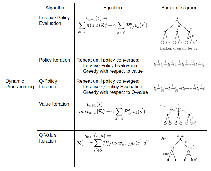
\[\begin{aligned} v_{k+1}(s) &= \sum_{a \in \mathcal{A}}\pi(a \vert s)[\mathcal{R}_{s}^{a} + \gamma \sum_{s^{'} \in S}\mathcal{P}_{ss^{'}}^{a}v_{k}(s^{'})]\\ \end{aligned}\]

Policy Iteration

Policy iteration consists of 2 steps. Given a policy, we evaluate given policy using policy evaluation from above and we act greedy with respect to value function obtained in policy evaluation step to get a improved policy. This step is called policy improvement step. We repeat these 2 steps until policy converges i.e there is no change in old and new improved policy.

where E denotes policy evaluation step and I denotes policy improvement step. This method converges to optimal value function (\(v_{*}\)) and optimal policy (\(\pi_{*}\)) in a finite number of iterations for a finite MDP. At convergence, we satisfy Bellman optimality equation for both policy and value function.

Generalized Policy Iteration

Policy Iteration consists of two process, policy evaluation making value function consistent with current policy and policy improvement making policy greedy with respect to the current value function. In generalized policy iteration(GPI), we perform continuous iterations of each policy evaluation and policy iteration alternatively. The value function is altered to more closely approximate the value function for the current policy, and the policy is repeatedly improved with respect to the current value function. Eventually both approximate value function and policy converges to optimal value function and optimal policy.

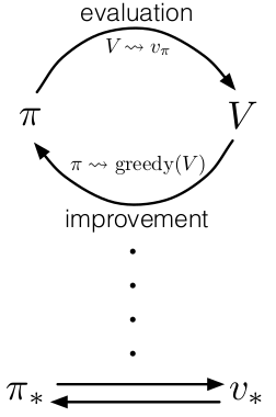
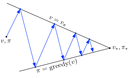
It’s sort of like tug-of-war, evaluation and improvement pull in opposing directions. If we make policy greedy with respect to current value function. In policy evaluation step, the value function will be incorrect for the changed policy. If we make value function consistent with the current policy, the current policy will no longer be greedy. This sort of war goes on between value function and policy trying to outsmart each other and eventually they stabilise to reach optimality.

Value Iteration

In policy iteration, we first evaluate a policy for some iterations and then move on to policy improvement step. What if we evaluate policy for 1 iteration? This will reduce the time we wait for value function to converge in policy evaluation step. This algorithm of policy evaluation for 1 iteration(update of each state) and policy improvement is called value iteration. We can combine the policy improvement and truncated policy evaluation steps in one equation. This equation turns Bellman optimality equation into update rule. This equation guarantees convergence to optimal value function similar to policy iteration. We keep track of policies in value iteration implicitly (take one step and choosing action that maximises expected reward). In value iteration, only a single iteration of policy evaluation is performed in between each policy improvement.

\[\begin{aligned} v_{k+1}(s) &= max_{a \in \mathcal{A}}[\mathcal{R}_{s}^{a} + \gamma \sum_{s^{'} \in S}\mathcal{P}_{ss^{'}}^{a}v_{k}(s^{'})]\\ \end{aligned}\]

There is another variant of iterative DP algorithms, Asynchronous DP where values of states are updated in any order whatsoever. DP algorithms are not practical for very large state space(or action space) because DP uses full-width backups. The number of deterministic policies for number of actions \(k\) and states \(n\) are \(n^{k}\). DP is exponentially faster than exhaustively searching each possible policy. All the DP algorithms seen above can be summarized in the table below.

Problem	Bellman Equation	Algorithm
Prediction	Bellman Expectation Equation	Iterative Policy Evaluation
Control	Bellman Expectation Equation + Greedy Policy Improvement	Policy Iteration
Control	Bellman Optimality Equation	Value Iteration

In DP, all of the estimate values for state where based on the estimates of values of successor states. In RL, this idea is called bootstrapping.

Model-free methods

To run model-based methods, we require full knowledge of MDP transitions. But sometimes environment can be unkind, keeping secrets from us. That’s when we turn to model-free methods. In model-free methods, we don’t have the complete dynamics of the environment. Hence, we interact with the environment to generate episodes of experience. In these methods, the model generates only sample transitions and not complete probability distribution of all possible transitions that is required for DP.

Monte Carlo

MC uses experiences, sample of sequences of states, actions, and rewards to estimate the average sample returns (not expected returns as seen in DP). As more returns are observed, the average should converge to the expected value. MC methods works only for episodic tasks. Each episode contains experiences and each episode eventually terminates. Only on the completion of an episode are value estimates and policies changed. This shows that MC methods are incremental learning methods, episode-by-episode sense but not in a step-by-step (online) sense. In MC like DP, we solve two problems of prediction and control. In MC prediction, given a policy we estimate state-value function or action-value function. In MC control, the goal is to find approximate optimal policy for an unknown MDP environment or a very large MDP environment.

There are two ways to solve MC control problem either on-policy or off-policy. For on-policy method, we estimate \(v_{\pi}\) (or \(q_{\pi}\)) for the current behaviour policy \(\pi\). For off-policy method, given two polices \(\pi\) and \(b\) we estimate \(v_{\pi}\) (or \(q_{\pi}\)) but all we have are episodes following from policy \(b\). The policy being learned about \(\pi\) is called target policy. The policy used to generate behaviour \(b\) is called behaviour policy.

First Visit

As seen in policy evaluation method, we wish to estimate \(v_{\pi}(s)\), given a set of episodes obtained by following \(\pi\) and passing through \(s\). Each occurrence of state \(s\) in an episode is called a visit to \(s\). With a model of MDP, we can estimate policy from values of states (taking one step and choose action that leads to the best combination of reward and next state). In first visit method, we estimate \(v_{\pi}(s)\) as the average of the returns following first visits to \(s\).

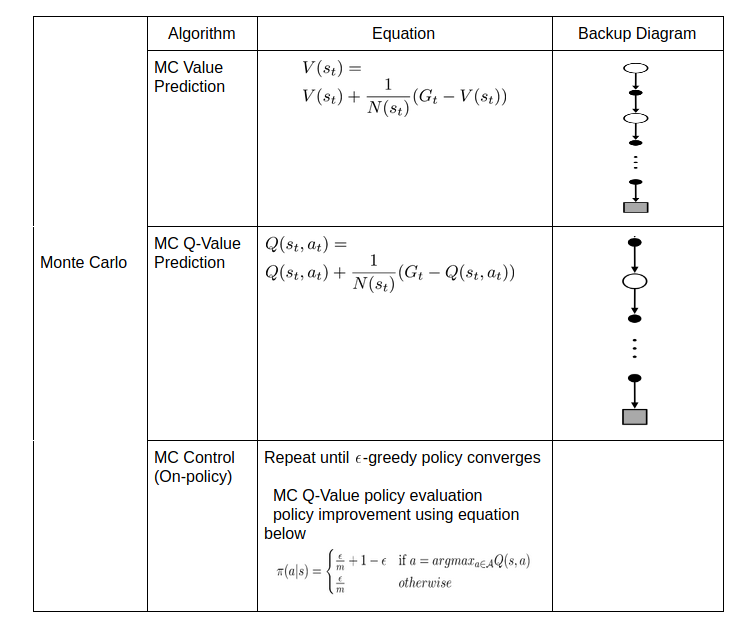
\[\begin{aligned} V(s_{t}) &= V(s_{t}) + \frac{1}{N(s_{t})}(G_{t} - V(s_{t}))\\ \end{aligned}\]

where \(G_{t}\) is total return from time step \(t\) and \(N(s_{t})\) keeps track of visits to state \(s_{t}\).

If we don’t have a model of MDP, the state values are not sufficient to provide a policy. In this case, we prefer to evaluate action-value \(q_{\pi}(s, a)\), the sample returns from taking action \(a\) from state \(s\) and following policy \(\pi\) thereafter. Estimating policy from action values is just taking argmax over the action values, choosing the action with highest action value. In first visit method, we estimate \(q_{\pi}(s, a)\) as the average of the returns following the first time in each episode that the state \(s\) was visited and the action \(a\) was selected.

Another variant of first visit is every visit. There can be multiple times state \(s\) can be visited in the same episode. So, instead of averaging returns of first visits to \(s\) in every visit we average the returns following all visits to state \(s\). Both first-visit MC and every-visit MC converge to \(v_{\pi}(s)\) as the number of visits (or first visits) to s goes to infinity.

On-policy MC Control

On-policy learning is like “learning on the job”.

In DP we saw that we can find optimal policy by using GPI. Similarly in MC, we use the same process for finding optimal policy. But one problem in MC control is that we don’t have a model of MDP. For value function policy evaluation methods from above either first visit or every visit method can be used to evaluate current policy. But when policy needs to be improved, we are expected to have transition probabilities over all actions from current state in choosing best action such that after taking one step using that action from current state and ending up in next state that will provide maximum returns. This is the reason why we prefer using action-values over state-values when dynamics of environment is not known. The policy for action action values is taking the action with maximum action value.

\[\begin{aligned} \pi^{'}(s) &= argmax_{a \in \mathcal{A}}[R^{a}_{s} + P^{a}_{ss^{'}}V(s^{'})]\\ &= argmax_{a \in \mathcal{A}}[Q(s, a)]\\ \end{aligned}\]

But there is a problem of exploration in dealing with action values. Many state–action pairs may never be visited. If our policy is deterministic policy, then in following that policy one will observe returns only for one of the actions from each state. The purpose of learning action values is to help in choosing among the actions available in each state. To solve this issue, we use a stochastic policy to ensure continual exploration. In \(\epsilon\)-greedy policy, most of the time they choose an action that has maximum estimated action value, but with probability \(\epsilon\) they instead select an action at random.

\[\begin{aligned} \pi(a \vert s) = \begin{cases} \frac{\epsilon}{m} + 1 - \epsilon &\mbox{if } a = argmax_{a \in \mathcal{A}}Q(s, a)\\ \frac{\epsilon}{m} & otherwise \end{cases} \end{aligned}\]

where \(m\) is all actions tried with non-zero probability.

We have a \(\epsilon\)-soft policy of choosing greedy action with probability \(1-\epsilon\) and choosing an action at random with probability \(\epsilon\). In on-policy, we continually estimate \(q_{\pi}\) for current behaviour policy \(\pi\) and at the same time make the policy \(\pi\) greedy with respect to \(q_{\pi}\).

Off-policy MC Control

Off-policy learning is like “learning from looking over someone’s shoulder”.

As observed in MC control, there is a trade-off between exploration and exploitation. The on-policy MC solves the problem of exploration by using \(\epsilon\)-greedy policy. In off-policy, we use two policies. One policy that is learn about and becomes optimal policy called target policy. One that is more exploratory and is used to generate behaviour called behaviour policy. MC uses importance sampling which we will explore in Extras blog (yet to be written).

TD Learning

TD Learning is a combination of ideas from DP and MC. Like DP, TD learning uses one-step look-ahead updates (bootstrapping) and like MC, TD methods can directly learn from experiences without the model of environment’s dynamics. TD methods are preferred over MC in environments where episodes do not terminate. Similar to above trend, we will solve two problem of prediction and control using TD methods. In TD prediction, given a policy we estimate state-value function or action-value function. In TD control, the goal is to find approximate optimal policy for an unknown MDP environment or a very large MDP environment. And similar to MC, TD control can be solved using two methods, on-policy and off-policy.

TD Prediction

Similar to MC, we use experiences to solve prediction problem. MC methods uses return to estimate the value of state and wait until the episode terminates to update the state value. TD on other hand updates its value towards one-step estimated return (\(R_{t+1} + \gamma V(s_{t+1})\)). This is called TD target. \(R_{t+1} + \gamma V(s_{t+1}) - V(s_{t})\) is called TD error as it measures the difference between the estimated value of \(s_{t}\) (\(V(s_{t})\)) and the better estimate \(R_{t+1} + \gamma V(s_{t+1})\). This learning a guess from a guess is known as bootstrapping. TD combines bootstrapping of DP with sampling of MC. For any fixed policy, \(V\) converges to \(v_{\pi}\).

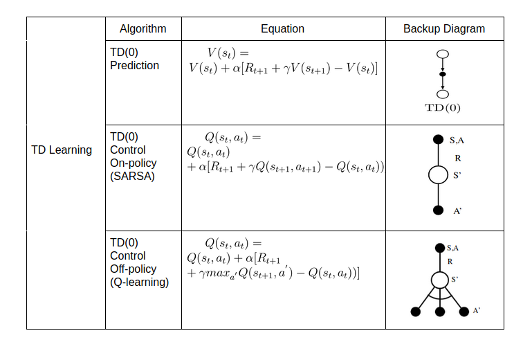
\[\begin{aligned} V(s_{t}) &= V(s_{t}) + \alpha [R_{t+1} + \gamma V(s_{t+1}) - V(s_{t})]\\ \end{aligned}\]

This method is also called TD(0), a special case of TD(\(\lambda\)), where instead of one-step returns, we use \((\lambda+1)\)-step returns to estimate the state-value function. TD methods are more biased towards next estimate than MC methods. They are more sensitive to initial values. There is less noise (variance) as compared to MC methods, where we take into consideration all the rewards until the episode terminates.

SARSA : On-policy TD Control

Without a given model, the goal is find optimal policy by learning state-action values. We consider transitions from state–action pair to state–action pair. An episode consists sequence of state-action pair (\((S, A)\)), immediate reward(\(R\)), next state(\(S^{'}\)) and next action(\(A^{'}\)), hence the name SARSA.

This seems a lot similar to on-policy MC Control where we wait until the episode terminates to estimate the return. But the only difference here is that we instead bootstrap to one-step estimated return. SARA converges \(Q(s, a)\) to \(q_{*}(s, a)\).

\[\begin{aligned} Q(s_{t}, a_{t}) &= Q(s_{t}, a_{t}) + \alpha [R_{t+1} + \gamma Q(s_{t+1}, a_{t+1}) - Q(s_{t}, a_{t}))]\\ \end{aligned}\]

Q-Learning : Off-policy TD Control

Q-learning is one of the most popular RL algorithms. In off-policy, we evaluate \(v_{\pi}\) (or \(q_{\pi}\)) for target policy \(\pi\) while following episodes generated from behaviour policy \(\mu\). In case of TD(0), the target policy will be greedy with respect to action-values and behaviour policy will be \(\epsilon\)-greedy with respect to action-values. We are balancing the greedy and exploration behaviour which we often observe in RL algorithms by using two policies.

\[\begin{aligned} Q(s_{t}, a_{t}) &= Q(s_{t}, a_{t}) + \alpha [R_{t+1} + \gamma max_{a^{'}} Q(s_{t+1}, a^{'}) - Q(s_{t}, a_{t}))]\\ \end{aligned}\]

This equation seems a lot familiar to Bellman optimality equations we seen above. Here, the alternate action \(a^{'}\) is chosen by the target policy and \(a_{t}\) is chosen according to behaviour policy. The next action to be updated is also chosen according to behaviour policy. We are updating the action values towards the best possible one-step action values. Q-learning converges to optimal action-value function.

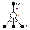
Backup Diagrams of DP, MC and TD

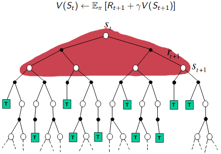
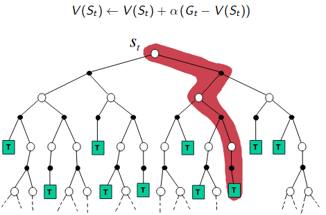
The backup diagrams of DP, MC and TD are compared in the table below.

DP Backup	MC Backup	TD Backup

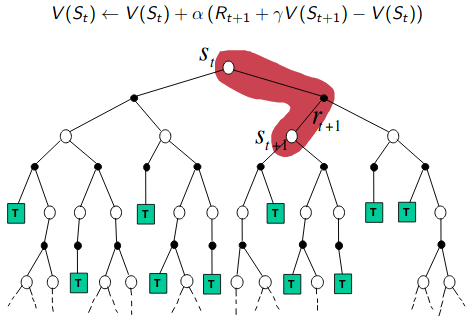If we compare the backup diagrams of all 3 algorithms, we can easily spot the difference. DP does a full-width shallow backup, MC does a sample deep backups and TD does a sample shallow backups.

Story so far

All of these equations might seem overwhelming. But all these algorithms sort of tell a story. We start with DP where we solve prediction and control problems. In DP, we know everything about the environment. We know what actions can be taken from current state with exact probabilities of taking particular action and the next possible states that we can end up in. We use this knowledge of transitions to solve prediction problem by evaluating a given policy by assigning a value(state or action) to a state(or action) equal to expected returns we can get from that state(or action) by following that policy. In control problem, we want to find the optimal policy i.e. what is the best action to take when in a state? We solve the control problem, by evaluating a policy like above and then improving the policy by making the policy greedy with respect to value function obtained in evaluating the policy. We continue this process of evaluation and improvement until policy no longer improves.

Next, we wonder what to do in case some environments are not so kind to provide us their inner working instead they provide us only the samples of sequences in form of episodes where each episode eventually terminates. Now instead of full known transitions, we work with samples of experience. In MC, we are required to solve prediction and control problem. In prediction problem, we evaluate a given policy by finding value estimates same as we did in DP. But we use first-visit or every-visit method. Nothing fancy, just we keep track of first visit and update the estimated returns until episode terminates or update the estimated returns from every visit of particular state. This shows that updates have more variance, a lot of noise. But when we move in solving control problem. We follow the same process of evaluating a policy and improving the policy to find optimal policy. To evaluate a given policy, instead of choosing to work with state-value functions for any of methods above (first-visit or every visit) we prefer using action-value function as the model is unknown i.e. if we want to obtain a policy from state-value functions, we need to do one-step look ahead over all states that can be visited from all actions that can be taken and choosing the action with maximum return. On contrary, devising a policy from action-values is just choosing action with maximum action-value. But there is another problem with action-values, not all pairs of (state, action) will be visited. So, to solve that we use \(\epsilon\)-greedy policy instead of greedy policy to encourage exploration. Now armed with these two modifications, we solve the control problem.

When we combine DP and MC, learning from bootstrapping and experience, we get TD. This is just like MC but instead of estimating returns until the episode terminates, we use one-step return estimate as done in DP. We learn online as we go. Similar to DP and MC, we solve prediction and control problem. In prediction problem, we use estimated returns from one-step instead of waiting till episode terminates as in case of MC. But the updates are more biased and low variance in case of TD, sensitive to initial values. The control problem can be solved in two ways either by on-policy or off-policy methods. In on-policy method, similar to MC control we use action-value updates and \(\epsilon\)-greedy policy but only difference being instead of returns from waiting until episode completes as in MC, we update the estimate based on returns from one-step estimated action-values. In off-policy, we use two policies (target and behaviour) to balance the exploration and exploitation. We make the current action values (chosen from behaviour policy) greedy with respect to maximum return from one-step estimated action values. This action value is chosen from target policy.

Another line of thought is, is there any way to get best of both worlds (MC and TD)? This is where n-step TD methods where we unify both TD and MC methods. But that’s a subject to be discussed in future Extras post(yet to be written).

We sum up everything we have visited using both the equations and backup diagrams in 3 tables shown below.

In next post, we will look into some of the ways we can avoid keeping large tables of action-values and state-values for solving the prediction and control problems of various RL algorithms.

Happy Learning!

Intuitions

State-value function : how good is it to be in a particular state

Action-value function : how good is to take a particular action in given state

Policy : what actions can I take when in a particular state

Prediction Problem : how good is this given policy

Control problem : what is the best policy from all the possible policies

Footnotes and Credits

RL Meme

Almost all figures are from RL book

Dopamine and temporal difference learning: A fruitful relationship between neuroscience and AI

NOTE

Questions, comments, other feedback? E-mail the author

Tabular Solution Methods

Tabular Solution Methods

Terminologies

Markov Process

Markov Reward Process

Markov Decision Process

Bellman Expectation Equation

Bellman Optimality Equation

Backup Diagrams

Tabular Solution Methods

Model-based methods

Dynamic Programming

Model-free methods

Monte Carlo

TD Learning

Backup Diagrams of DP, MC and TD

Story so far

Intuitions

Further Reading

Footnotes and Credits