MLP
In this post, we will go through basics of MLP using MNIST dataset. We will implement this using two popular deep learning frameworks Keras and PyTorch.
All the codes implemented in Jupyter notebook in Keras, PyTorch, Tensorflow and fastai.
All codes can be run on Google Colab (link provided in notebook).
Hey yo, but what is MLP? what is MNIST?
Well sit tight and buckle up. I will go through everything in-detail.

Feel free to jump anywhere,
# load all the required libraries

import numpy as np                                    # package for computing
from sklearn.model_selection import train_test_split  # split dataset
import keras                                          # import keras with tensorflow as backend
from keras.datasets import mnist                      # import mnist dataset from keras
from keras.models import Model, Sequential            # sequential and functional api keras
from keras.layers import Dense, Input                 # dense and input layer for constructing mlp

import matplotlib.pyplot as plt             # matplotlib library for plotting

# display plots inline (in notebook itself)

%matplotlib inline
Using TensorFlow backend.
MNIST Dataset
The MNIST dataset of handwritten digits has a training set of 60,000 examples, and a test set of 10,000 examples each of size 28 x 28 pixels. The digits have been size-normalized and centered in a fixed-size image.
It is a good database for people who want to try learning techniques and pattern recognition methods on real-world data while spending minimal efforts on preprocessing and formatting.
Here is one example of number 5 from dataset

# load mnist data

# the data, split between train and validation sets
(train_x, train_y), (test_x, test_y) = mnist.load_data()

#orginally shape (60000, 28, 28) for train and (10000, 28, 28) for test
#but as we will be using fully connected layers we will flatten
#the images into 1d array of 784 values instead of (28 x 28) 2d array
train_x = train_x.reshape(60000, 784)
test_x = test_x.reshape(10000, 784)

# As image is grayscale it has values from [0-255] which we will visualize below
# convert dtype to float32 and scale the data from [0-255] to [0-1]
train_x = train_x.astype('float32')
test_x = test_x.astype('float32')
train_x /= 255
test_x /= 255

print('Training samples and shape:', train_x.shape[0], train_x.shape)
print('Test samples and shape:', test_x.shape[0], test_x.shape)
Downloading data from https://s3.amazonaws.com/img-datasets/mnist.npz
11493376/11490434 [==============================] - 0s 0us/step
Training samples and shape: 60000 (60000, 784)
Test samples and shape: 10000 (10000, 784)
Different sets of splitting data
Wait hold on second, what are these different sets?
We usually define
- Training set - which you run your model (or learning) algorithm on.
- Dev (development) or val (validation) set - which you use to tune parameters, select features, and make other decisions regarding learning algorithms or model. Sometimes also called out as hold-out cross validation set
- Test set - which you use to evaluate the performance of algorithm, but not to make any decisions regarding what the model or learning algorithm or parameters to use.
The dev and test set allow us to quickly see how well our model is doing.
Cat Classifier
Consider a scenario where we are building cat classifier (cats really, why not!). We run a mobile app, and users are uploading pictures of many different things to the app.

We collect a large training set by downloading pictures of cats (positive examples) and non-cats (negative examples) off of different websites. We split the dataset 70% / 30% into training and test sets. Using this data, we build a cat detector that works well on the training and test sets. But when we deploy this classifier into the mobile app, we find that the performance is really poor!
What happened?
Since training/test sets were made of website images, our algorithm did not generalize well to the actual distribution you care about: mobile phone pictures.
Before the modern era of big data, it was a common rule in machine learning to use a random 70% / 30% split to form training and test sets. This practice can work, but it’s a bad idea in more and more applications where the training distribution (website images in our example above) is different from the distribution you ultimately care about (mobile phone images).
Lesson: Choose dev and test sets to reflect data you expect to get in the future and want to do well on.
# we will split val into --> 20% val set and 80% test set
# stratify ensures the distribution of classes is same in both the sets

val_x, test_x, val_y, test_y = train_test_split(test_x, test_y, test_size=0.8, stratify=test_y)

print ('Validation samples and shape', val_x.shape[0], val_x.shape)
print ('Test samples and shape', test_x.shape[0], test_x.shape)
Validation samples and shape 2000 (2000, 784)
Test samples and shape 8000 (8000, 784)
Visualization of data
Enough talk, show me the data!
# plot the images in the batch, along with the corresponding labels
fig = plt.figure(figsize=(25, 4))

for idx in np.arange(20):
    ax = fig.add_subplot(2, 20/2, idx+1, xticks=[], yticks=[])
    ax.imshow(train_x[idx].reshape(28, 28), cmap='gray')
    # print out the correct label for each image
    ax.set_title(str(train_y[idx]))

img = train_x[1].reshape(28, 28)

fig = plt.figure(figsize = (12,12))
ax = fig.add_subplot(111)
ax.imshow(img, cmap='gray')
width, height = img.shape
thresh = img.max()/2.5
for x in range(width):
    for y in range(height):
        val = round(img[x][y],2) if img[x][y] !=0 else 0
        ax.annotate(str(val), xy=(y,x),
                    horizontalalignment='center',
                    verticalalignment='center',
                    color='white' if img[x][y]<thresh else 'black')
Introduction to MLP
MLP is multi-layer percepton. Perceptron is a single layer neural network and a multi-layer perceptron is called Neural Networks.
We have seen the dataset, which consist of [0-9] numbers and images of size 28 x 28 pixels of values in range [0-1] .
Now, I-know-nothing being too lazy to find which number is what asks for I-know-everything apprenticeship to create a Machine Learning Model such that if we pass a grayscale image of size 28 x 28 pixels to the model, it outputs a correct label corresponding to that image.

A long time ago in a galaxy far, far away….
I-know-nothing: Master, how can I create such a intelligent machine to recognize and label given images?
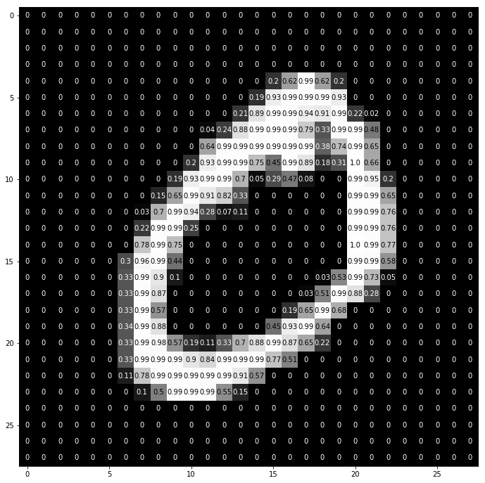
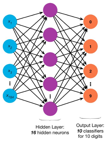
I-know-everything: Young Padwan, we will use the Force of Neural Networks inspired from our brain. Here, let me take you on a journey of one example for example 0. We have 784 pixel values in range [0-1] describing what zero looks like (pixels bright in the center in shape of 0 and dark like the dark side elsewhere). Have a look at 0 example above. 0 passes through the network like the one shown below and return 10 values which will help in classfying the image is 0 or 1 or 2 and so on.
I-know-nothing: How will the network decide which image is what label?
I-know-everything: If the image passed is 0 (also known as forward pass), the network will output array [1, 0, 0, 0, 0, 0, 0, 0, 0, 0]. The first place 1 indicates the image passed is 0, hence label 0.
I-know-nothing: How does the network learn such a magic trick?
I-know-everything: Young Padwan, you are learning to ask right questions. I will give 2 explainations so listen closely. First let me give you an intuitive explaination. The neural networks train themselves repetitively on data so that they can adjust the weights in each layer of the network to get the final result closer to given label by minimizing loss function. Now the second explaination in jargon words, as shown in the network we have input layer, hidden layer and output layer. Okay? So, input layer has 784 nodes (neurons) i.e. it accepts 784 values which is exactly what our example 0 has. Next node is hidden layer which contains 16 neuron and what are its values? They are randomly initialized. This random intialization also plays a critical role, we can’t just set all values to 0 or very high values as they can get us into trouble like vanishing gradient or exploding gradients. We will explore this term more in our LSTM post. There are many initialization techniques like He initialization, Xavier initialization, etc. Next is the output layer which has 10 nodes. These are the values which our network gives us after performing special operations which then we will compare to our desired label which is zero in this case.
I-know-nothing: What if network outputs does not match our desired result?
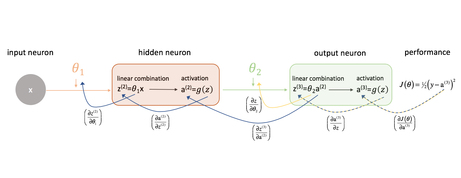
I-know-everything: That means, our network is stupid (for now). But it learns, it learns from its mistakes. The process by which it learns is backpropagation. So, in jar jar backpropagation, in our example desired result was [1, 0, 0, 0, 0, 0, 0, 0, 0, 0] and network outputs [0.24, 0.542, 0.121, 0.32, 0.56, 0.67, 0.213, 0.45, 0.312, 0.98] which in this case is 9 (highest value). So, now network tells its previous layer (process also known as backward pass), hidden layer hey look you gave me wrong answer 9, see here the right answer was 0 which is called as loss. Make necessary changes with help of chain rule to your weights so that when next time you see 0, you will improve the prediction in such a way that output will be correct label 0.

I-know-nothing: Does repeating these telling, the correct results and correcting the wrong results is what Force of Neural Networks all about?
I-know-everything: Well, if you put it that way, you are sucking all the fun out of magic. But yes, this is what is called supervised learning, where network is supervised to show it direction so that it does not get lost in the woods (Out of Woods).
I-know-nothing: This is all intutive understanding with some jargon words. What about real equations? I mean, everywhere I see there are equations. Where are they?
I-know-everything: They are bit scary but if you insist I will write them for you.

Forward Pass
\[\begin{aligned} \mathbf{a} & = \mathbf{w\rm\normalsize i^T} \mathbf{x} + \mathbf{w\rm\normalsize i_0} \\ \mathbf{h} & = f(\mathbf{a}) = f(\mathbf{w\rm\normalsize i^T} \mathbf{x} + \mathbf{w\rm\normalsize i_0}) \\ \mathbf{z} & = \mathbf{w\rm\normalsize o^T} \mathbf{h} + \mathbf{w\rm\normalsize o_0} \\ \mathbf{\hat{y}} & = softmax(\mathbf{z}) \\ \\~\\ \textrm{Relu Non-linearity}: f(\mathbf{k}) & = max(k, 0) \\ \textrm{Softmax Function}: \sigma_j(\mathbf{z}) & = \frac {\exp(\mathbf{z}_j)} {\sum_{k}^{nclass} \exp(\mathbf{z}_k)} \\ \end{aligned}\]Error Function
\[\begin{aligned} E = l(\mathbf{y}, \mathbf{\hat{y}}) = -\sum_{i}^{nclass}\mathbf{y_i}ln{\mathbf{\hat{y_i}}} \end{aligned}\]Backward Pass
\[\begin{aligned} \frac{\partial E}{\partial \mathbf{\hat{y_i}}} & = - \frac {\mathbf{y_i}}{\mathbf{\hat{y_i}}} \\ \frac{\partial \mathbf{\hat{y_i}}}{\partial \mathbf{z}} & = \begin{cases} & \frac {\exp(\mathbf{z}_i)} {\sum_{k}^{nclass} \exp(\mathbf{z}_k)} - (\frac {\exp(\mathbf{z}_i)} {\sum_{k}^{nclass} \exp(\mathbf{z}_k)})^2 &i=k \\ & (\frac {e^{(\mathbf{z}_i)}e^{(\mathbf{z}_k)}} {\sum_{k}^{nclass} \exp(\mathbf{z}_k)})^2 & i \ne k \\ & \end{cases} \\ &= \begin{cases} \mathbf{\hat{y_i}}(1-\mathbf{\hat{y_i}}) &i=k \\ -\mathbf{\hat{y_i}}\mathbf{\hat{y_k}} &i \ne k \\ \end{cases} \\ \frac{\partial E}{\partial \mathbf{z_i}} & = \sum_{k}^{class}\frac{\partial E}{\partial \mathbf{\hat{y_k}}}\frac{\partial \mathbf{\hat{y_k}}}{\partial \mathbf{z_i}} \\ & = \frac{\partial E}{\partial \mathbf{\hat{y_i}}}\frac{\partial \mathbf{\hat{y_i}}}{\partial \mathbf{z_i}} - \sum_{i \ne k}\frac{\partial E}{\partial \mathbf{\hat{y_k}}}\frac{\partial \mathbf{\hat{y_k}}}{\partial \mathbf{z_i}} \\ & = \sum_{k}^{class}\frac{\partial E}{\partial \mathbf{\hat{y_i}}}\frac{\partial \mathbf{\hat{y_i}}}{\partial \mathbf{z_i}} \\ & = -\mathbf{\hat{y_i}}(1-\mathbf{y_i}) + \sum_{k \ne i}\mathbf{\hat{y_k}}\mathbf{y_i} \\ & = -\mathbf{\hat{y_i}} + \mathbf{y_i}\sum_{k}\mathbf{\hat{y_k}} \\ & = \mathbf{\hat{y_i}} - \mathbf{y_i} \\ \frac{\partial E}{\partial \mathbf{w\rm\normalsize o_{ji}}} & = \sum_{i}\frac{\partial E}{\partial \mathbf{z_i}}\frac{\partial \mathbf{z_i}}{\partial \mathbf{w\rm\normalsize o_{ji}}} \\ & = (\mathbf{\hat{y_i}} - \mathbf{y_i})\mathbf{h_j} \\ \frac{\partial E}{\partial \mathbf{w\rm\normalsize o_{0}}} & = \frac{\partial E}{\partial \mathbf{z_i}} = \mathbf{\hat{y_i}} - \mathbf{y_i} \\ \frac{\partial E}{\partial \mathbf{h_{ji}}} & = \sum_{i}\frac{\partial E}{\partial \mathbf{z_i}}\frac{\partial \mathbf{z_i}}{\partial \mathbf{h_{ji}}} \\ & = (\mathbf{\hat{y_i}} - \mathbf{y_i})\mathbf{w\rm\normalsize o_j} \\ \frac{\partial \mathbf{h_{ji}}}{\partial \mathbf{a}} & = \begin{cases} 1 &a>0 \\ 0 &else \\ \end{cases} \\ \frac{\partial E}{\partial \mathbf{w\rm\normalsize i_{ji}}} & = \sum_{i}\frac{\partial E}{\partial \mathbf{h_{ji}}}\frac{\partial \mathbf{h_{ji}}}{\partial \mathbf{a}}\frac{\partial \mathbf{a}}{\partial \mathbf{w\rm\normalsize i_{ji}}} \\ & = (\mathbf{\hat{y_i}} - \mathbf{y_i})\mathbf{w\rm\normalsize o_j}\mathbf{x\rm\normalsize _j} \\ \frac{\partial E}{\partial \mathbf{w\rm\normalsize i_{0}}}& =\frac{\partial E}{\partial \mathbf{h_{ji}}} = (\mathbf{\hat{y_i}} - \mathbf{y_i})\mathbf{w\rm\normalsize o_j} \\ \end{aligned}\]Here is how all the equations of matrix multiplications pan out for our example.
Input (i) -> (784 x 1) -> 784 neurons
Hidden Layer (w) -> (16 x 784) -> 16 neurons
Output Layer (o) -> (10 x 16) -> 10 neurons
Bias hidden (bh) -> (16 x 1)
Bias output (bo) -> (10 x 1)
h = matrix_mulitiplication(w, i) + bh -> resulting dimension (16 x 1)
y_ = matrix_mulitiplication(o, h) + bo -> resulting dimension (10 x 1)
y_ = softmax(y_) -> same dimension (10 x 1) just squashing everything between 0 and 1 such that all 10 values sum upto value 1.
Here we get our predicted output y_ which is compared with correct y through Loss function L, to get error.
Error (E) = Loss_Function(y, y_)
This Error (E) is the backpropagated from output layer through hidden layer to input layer.
I-know-everything: I am sure you got lot of questions now. So, shoot.
I-know-nothing: Wow! That’s mouthful! What is \(\mathbf{w\rm\normalsize i_{0}}\) and \(\mathbf{w\rm\normalsize o_{0}}\)? What is the function \(f(\mathbf{h})\) ? What are we doing in backpropagation? Is backpropagation only the way to propogate calculate error?
I-know-everything: Wooh slow down! Okay let’s answer it one by one.
- What is \(\mathbf{w\rm\normalsize i_{0}}\) and \(\mathbf{w\rm\normalsize o_{0}}\)?
These are called biases. A layer in a neural network without a bias is nothing more than the multiplication of an input vector with a matrix. Using a bias, you’re effectively adding another dimension to your input space.
- What is the function \(f(\mathbf{h})\)?
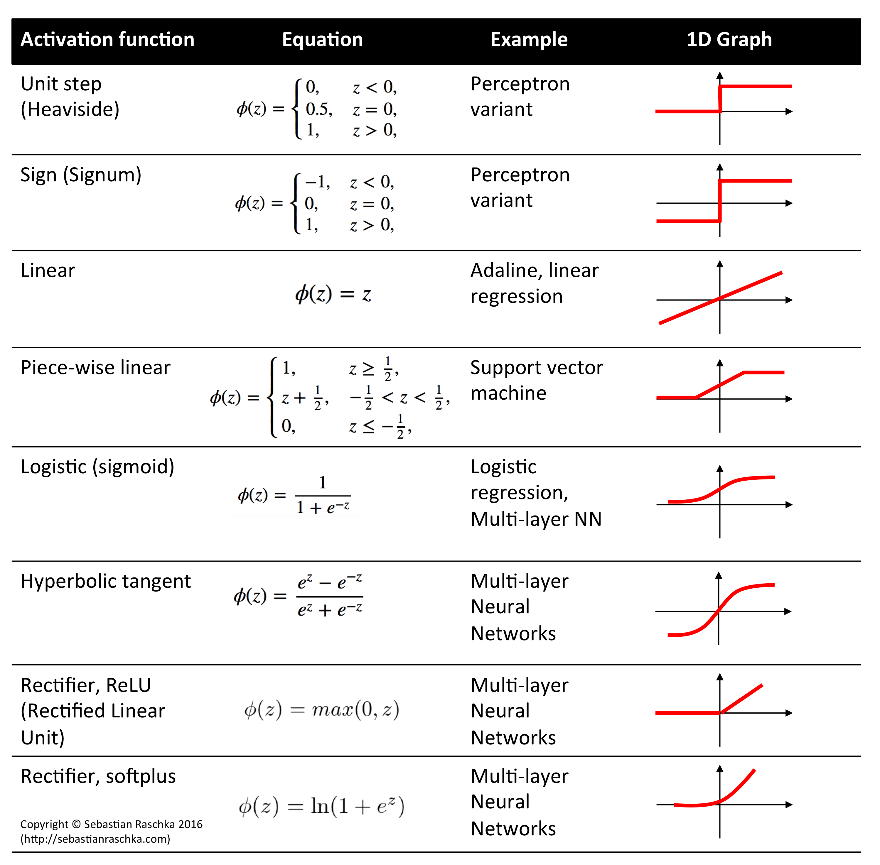
This functon plays an important role in machine learning. This types function are called non-linear functions. By introducing them in our network we introduce non-linearlity, non-linear means that the output cannot be reproduced from a linear combination of the inputs. Another way to think of it is if we don’t use a non-linear activation function in the network, no matter how many layers it had, the network would behave just like a single-layer perceptron, because summing these layers would give you just another linear function and most of the problems in real world are non-linear. Non-linearity is needed in activation functions because its aim in a neural network is to produce a nonlinear decision boundary via non-linear combinations of the weight and inputs. To provide a better seperation for higher dimensional data then a simple line seperator using linear function. There are several types of non-linear functions.
- What are we doing in backprop and is it the only way?
While designing a Neural Network, in the beginning, we initialize weights with some random values or any variable for that fact. So, it’s not necessary that whatever weight values we have selected will be correct, or it fits our model the best. Okay, fine, we have selected some weight values in the beginning, but our model output is way different than our actual output i.e. the error value is huge.
Now, how will you reduce the error?
Basically, what we need to do, we need to somehow explain the model to change the parameters (weights), such that error becomes minimum. That means, we need to train our model. One way to train our model is through Backpropagation but it is not the only way. There is another method called Synthetic Gradient designed by the Jedi Council of DeepMind. We will visit them later. If you are curious, look them up here and here.
In short, backprop algorithm looks for the minimum value of the error function in weight space using a technique called gradient descent. The weights that minimize the error function is then considered to be a solution to the learning problem.
Gradient Descent is like descending a mountain blind folded. And goal is to come down from the mountain to the flat land without assistance. The only assistance you have is a gadget which tells you the height from sea-level. What would be your approach be. You would start to descend in some random direction and then ask the gadget what is the height now. If the gadget tells you that height and it is more than the initial height then you know you started in wrong direction. You change the direction and repeat the process. This way in many iterations finally you successfully descend down.
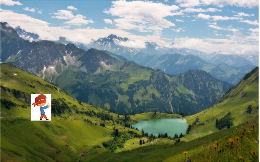
This is what gradient descent does. It tells the model which direction to move to minimize the error. There are different optimizer which tell us how can we find this direction.
a. Vanilla Gradient or Gradient Descent
b. Adam
c. RMSprop
d. Stochastic Gradient Descent(SGD)
e. Nesterov accelerated gradient (NAG)
f. Adadelta
g. Adagrad
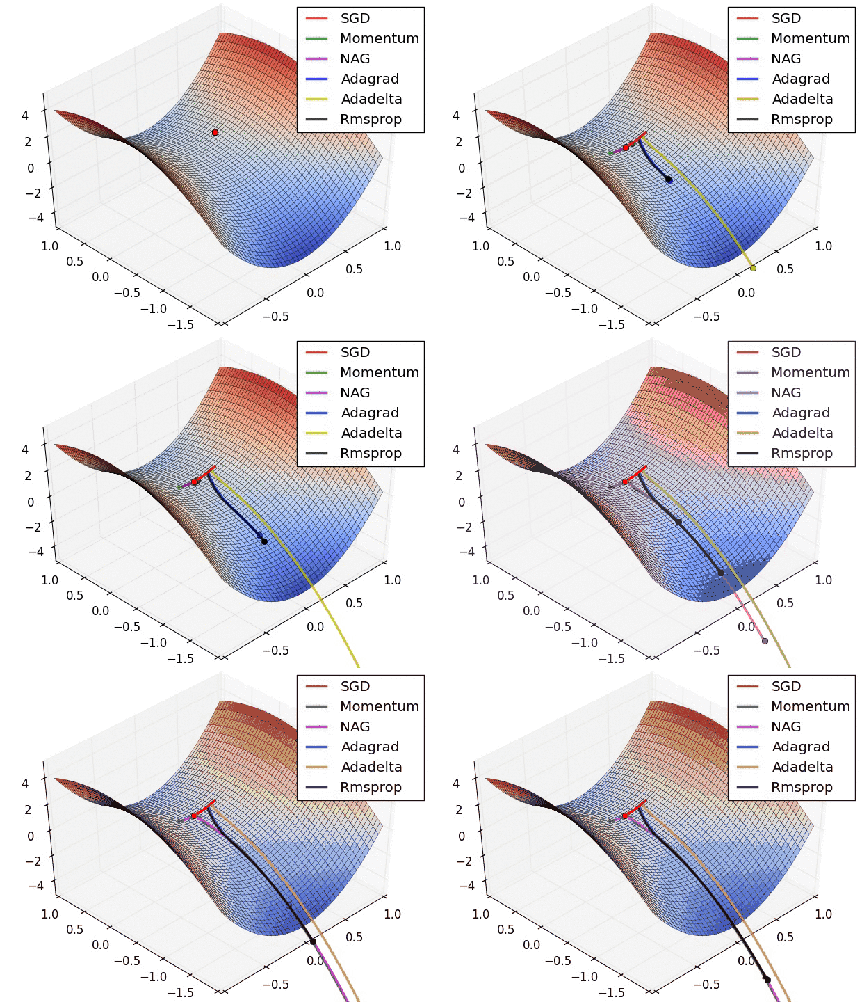
And this is behind the scenes (BTS) of how a Force of Neural Network learns.
I-know-nothing: Thank you Master, I follow.
I-know-everything: Now you are in for a treat. As you have learn about what different terms and functions are used to train a neural network. We will dive-in implementation using Keras. Here backpropagation is already implemented i.e. you only need to design forward pass and loss(or error) function, the framework does the heavy lifting to calculate backward pass and propogate it to all layers.
Recap
- We looked into what is MLP
- What are different layers in MLP
- What is forward propogation and backward propogation(pass) and how each of them work
- What is meant by training a neural network or in this case MLP
- How does neural network learn to classify images
- Scary backprop equations, loss function and role of biases
- Different types of activation functions and role of non-linear functions like ReLu, Sigmoid, etc
- Role of optimizers
- Different types of optimization algorithms required to train NN
Keras
Keras Sequential API
# [0-9] unique labels
num_classes = 10
epochs = 5
batch_size = 32
# convert class vectors to binary class matrices
train_y = keras.utils.to_categorical(train_y, num_classes)
val_y = keras.utils.to_categorical(val_y, num_classes)
test_y = keras.utils.to_categorical(test_y, num_classes)
print ('Training labels shape:', train_y.shape)
Training labels shape: (60000, 10)
model = Sequential()
model.add(Dense(784, activation='relu', input_shape=(784,)))
model.add(Dense(16, activation='relu'))
model.add(Dense(num_classes, activation='softmax'))

model.summary()

model.compile(loss='categorical_crossentropy',
              optimizer='Adam',
              metrics=['accuracy'])
_________________________________________________________________
Layer (type)                 Output Shape              Param #
=================================================================
dense_1 (Dense)              (None, 784)               615440
_________________________________________________________________
dense_2 (Dense)              (None, 16)                12560
_________________________________________________________________
dense_3 (Dense)              (None, 10)                170
=================================================================
Total params: 628,170
Trainable params: 628,170
Non-trainable params: 0
_________________________________________________________________
history = model.fit(train_x, train_y,
                    batch_size=batch_size,
                    epochs=epochs,
                    verbose=1,
                    validation_data=(val_x, val_y))
Train on 60000 samples, validate on 2000 samples
Epoch 1/5
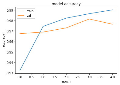
60000/60000 [==============================] - 45s 754us/step - loss: 0.2280 - acc: 0.9324 - val_loss: 0.1070 - val_acc: 0.9675
Epoch 2/5
60000/60000 [==============================] - 45s 754us/step - loss: 0.0858 - acc: 0.9744 - val_loss: 0.0932 - val_acc: 0.9690
Epoch 3/5
60000/60000 [==============================] - 45s 751us/step - loss: 0.0574 - acc: 0.9823 - val_loss: 0.0877 - val_acc: 0.9730
Epoch 4/5
60000/60000 [==============================] - 48s 804us/step - loss: 0.0413 - acc: 0.9866 - val_loss: 0.0606 - val_acc: 0.9815
Epoch 5/5
60000/60000 [==============================] - 50s 834us/step - loss: 0.0299 - acc: 0.9903 - val_loss: 0.0791 - val_acc: 0.9765
# summarize history for accuracy
plt.plot(history.history['acc'])
plt.plot(history.history['val_acc'])
plt.title('model accuracy')
plt.ylabel('accuracy')
plt.xlabel('epoch')
plt.legend(['train', 'val'], loc='upper left')
plt.show()
# summarize history for loss
plt.plot(history.history['loss'])
plt.plot(history.history['val_loss'])
plt.title('model loss')
plt.ylabel('loss')
plt.xlabel('epoch')
plt.legend(['train', 'val'], loc='upper left')
plt.show()

score = model.evaluate(test_x, test_y, verbose=0)
print('Test loss:', score[0])
print('Test accuracy:', score[1])
Test loss: 0.0735809408277
Test accuracy: 0.97975
# obtain one batch of test images
images, labels = test_x[:32], test_y[:32]

# get sample outputs
predict = model.predict_on_batch(images)
# convert output probabilities to predicted class
preds = np.argmax(predict, axis=1)
labels = np.argmax(labels, axis=1)

# plot the images in the batch, along with predicted and true labels
fig = plt.figure(figsize=(25, 4))
for idx in np.arange(20):
    ax = fig.add_subplot(2, 20/2, idx+1, xticks=[], yticks=[])
    ax.imshow(images[idx].reshape((28, 28)), cmap='gray')
    ax.set_title("{} ({})".format(str(preds[idx]), str(labels[idx])),
                 color=("green" if preds[idx]==labels[idx] else "red"))

Keras Functional API
# [0-9] unique labels
num_classes = 10
epochs = 5
batch_size = 32
inputs = Input(shape=(784,))
x = Dense(784, activation='relu')(inputs)
x = Dense(16, activation='relu')(x)
predictions = Dense(num_classes, activation='softmax')(x)

model = Model(inputs=inputs, outputs=predictions)

model.compile(loss='categorical_crossentropy',
              optimizer='Adam',
              metrics=['accuracy'])
history = model.fit(train_x, train_y,
                    batch_size=batch_size,
                    epochs=epochs,
                    verbose=1,
                    validation_data=(val_x, val_y))
Train on 60000 samples, validate on 2000 samples
Epoch 1/5
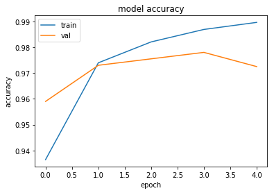
60000/60000 [==============================] - 49s 816us/step - loss: 0.2154 - acc: 0.9365 - val_loss: 0.1260 - val_acc: 0.9590
Epoch 2/5
60000/60000 [==============================] - 48s 801us/step - loss: 0.0833 - acc: 0.9740 - val_loss: 0.0766 - val_acc: 0.9730
Epoch 3/5
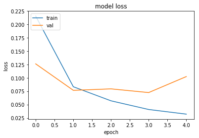
60000/60000 [==============================] - 48s 794us/step - loss: 0.0570 - acc: 0.9821 - val_loss: 0.0793 - val_acc: 0.9755
Epoch 4/5
60000/60000 [==============================] - 45s 757us/step - loss: 0.0408 - acc: 0.9869 - val_loss: 0.0724 - val_acc: 0.9780
Epoch 5/5
60000/60000 [==============================] - 44s 740us/step - loss: 0.0321 - acc: 0.9896 - val_loss: 0.1023 - val_acc: 0.9725
# summarize history for accuracy
plt.plot(history.history['acc'])
plt.plot(history.history['val_acc'])
plt.title('model accuracy')
plt.ylabel('accuracy')
plt.xlabel('epoch')
plt.legend(['train', 'val'], loc='upper left')
plt.show()
# summarize history for loss
plt.plot(history.history['loss'])
plt.plot(history.history['val_loss'])
plt.title('model loss')
plt.ylabel('loss')
plt.xlabel('epoch')
plt.legend(['train', 'val'], loc='upper left')
plt.show()
score = model.evaluate(test_x, test_y, verbose=0)
print('Test loss:', score[0])
print('Test accuracy:', score[1])
# obtain one batch of test images
images, labels = test_x[:32], test_y[:32]

# get sample outputs
predict = model.predict_on_batch(images)
# convert output probabilities to predicted class
preds = np.argmax(predict, axis=1)
labels = np.argmax(labels, axis=1)

# plot the images in the batch, along with predicted and true labels
fig = plt.figure(figsize=(25, 4))
for idx in np.arange(20):
    ax = fig.add_subplot(2, 20/2, idx+1, xticks=[], yticks=[])
    ax.imshow(images[idx].reshape((28, 28)), cmap='gray')
    ax.set_title("{} ({})".format(str(preds[idx]), str(labels[idx])),
                 color=("green" if preds[idx]==labels[idx] else "red"))

PyTorch
# load all the required libraries
import time
import copy
import numpy as np                                    # package for computing
from torch.utils.data.sampler import SubsetRandomSampler # split dataset
import torch                                          # import torch
from torchvision import datasets                      # import dataset from torch
import torchvision.transforms as transforms           # apply transformations to data
import torch.nn as nn                                 # neural network modules
import torch.nn.functional as F                       # functional api
from torch import optim                               # optimizers

# Detect if we have a GPU available
device = torch.device("cuda:0" if torch.cuda.is_available() else "cpu")

import matplotlib.pyplot as plt             # matplotlib library for plotting

# display plots inline (in notebook itself)
%matplotlib inline
# load mnist data

# number of subprocesses to use for data loading
num_workers = 0

# how many samples per batch to load
batch_size = 20

# percentage of training set to use as validation
val_size = 0.2

# convert data to torch.FloatTensor
transform = transforms.ToTensor()

# choose the training and test datasets
train_data = datasets.MNIST(root='data', train=True,
                                   download=True, transform=transform)
test_data = datasets.MNIST(root='data', train=False,
                                  download=True, transform=transform)

# obtain training indices that will be used for validation
num_test = len(test_data)
indices = list(range(num_test))
np.random.shuffle(indices)
split = int(np.floor(val_size * num_test))
test_idx, val_idx = indices[split:], indices[:split]

# define samplers for obtaining training and validation batches
test_sampler = SubsetRandomSampler(test_idx)
val_sampler = SubsetRandomSampler(val_idx)

# prepare data loaders (combine dataset and sampler)
train_loader = torch.utils.data.DataLoader(train_data, batch_size=batch_size,
                                           num_workers=num_workers)
val_loader = torch.utils.data.DataLoader(test_data, batch_size=batch_size,
                                         sampler=val_sampler, num_workers=num_workers)
test_loader = torch.utils.data.DataLoader(test_data, batch_size=batch_size,
                                          sampler=test_sampler, num_workers=num_workers)

print ('Training samples:', len(train_loader.dataset))
print ('Validation samples:', len(val_loader.dataset))
print ('Testing samples:',len(test_loader.dataset))

# Create training and validation dataloaders
dataloaders_dict = {'train': train_loader,
                    'val': val_loader}
Training samples: 60000
Validation samples: 10000
Testing samples: 10000
Visualization of data
import matplotlib.pyplot as plt
%matplotlib inline

# obtain one batch of training images
dataiter = iter(train_loader)
images, labels = dataiter.next()
images = images.numpy()

# plot the images in the batch, along with the corresponding labels
fig = plt.figure(figsize=(25, 4))
for idx in np.arange(20):
    ax = fig.add_subplot(2, 20/2, idx+1, xticks=[], yticks=[])
    ax.imshow(np.squeeze(images[idx]), cmap='gray')
    # print out the correct label for each image
    # .item() gets the value contained in a Tensor
    ax.set_title(str(labels[idx].item()))

img = np.squeeze(images[1])

fig = plt.figure(figsize = (12,12))
ax = fig.add_subplot(111)
ax.imshow(img, cmap='gray')
width, height = img.shape
thresh = img.max()/2.5
for x in range(width):
    for y in range(height):
        val = round(img[x][y],2) if img[x][y] !=0 else 0
        ax.annotate(str(val), xy=(y,x),
                    horizontalalignment='center',
                    verticalalignment='center',
                    color='white' if img[x][y]<thresh else 'black')

PyTorch Sequential API
# [0-9] unique labels
num_classes = 10
epochs = 5
## Define the NN architecture
class Net(nn.Module):
    def __init__(self):
        super(Net, self).__init__()
        D_in = 784
        H = 16
        D_out = num_classes
        self.classifier = torch.nn.Sequential(
            torch.nn.Linear(D_in, H),
            torch.nn.ReLU(),
            torch.nn.Linear(H, D_out),
            torch.nn.LogSoftmax(dim=1)
        )

    def forward(self, x):
        # flatten image input
        x = x.view(-1, 28 * 28)
        # 1 hidden layer, with relu activation function
        x = self.classifier(x)
        return x

# initialize the NN
model = Net()
model = model.to(device)
print(model)
Net(
  (classifier): Sequential(
    (0): Linear(in_features=784, out_features=16, bias=True)
    (1): ReLU()
    (2): Linear(in_features=16, out_features=10, bias=True)
    (3): LogSoftmax()
  )
)
# specify loss function
criterion = nn.NLLLoss()

# specify optimizer
optimizer = optim.Adam(model.parameters(), lr=1e-3)
def train_model(model, dataloaders, criterion, optimizer, num_epochs):
    since = time.time()

    history = dict()

    best_model_wts = copy.deepcopy(model.state_dict())
    best_acc = 0.0

    for epoch in range(num_epochs):
        print('Epoch {}/{}'.format(epoch, num_epochs - 1))
        print('-' * 10)

        # Each epoch has a training and validation phase
        for phase in ['train', 'val']:
            if phase == 'train':
                model.train()  # Set model to training mode
            else:
                model.eval()   # Set model to evaluate mode

            running_loss = 0.0
            running_corrects = 0

            # Iterate over data.
            for inputs, labels in dataloaders[phase]:
                inputs = inputs.to(device)
                labels = labels.to(device)

                # zero the parameter gradients
                optimizer.zero_grad()

                # forward
                # track history if only in train
                with torch.set_grad_enabled(phase == 'train'):
                    # Get model outputs and calculate loss

                    # backward + optimize only if in training phase
                    if phase == 'train':
                        outputs = model(inputs)
                        loss = criterion(outputs, labels)
                        loss.backward()
                        optimizer.step()

                    else:
                        outputs = model(inputs)
                        loss = criterion(outputs, labels)

                    _, preds = torch.max(outputs, 1)

                # statistics
                running_loss += loss.item() * inputs.size(0)
                running_corrects += torch.sum(preds == labels.data)

            epoch_loss = running_loss / (len(dataloaders[phase])*batch_size)
            epoch_acc = running_corrects.double() / (len(dataloaders[phase])*batch_size)

            print('{} Loss: {:.4f} Acc: {:.4f}'.format(phase, epoch_loss, epoch_acc))
            print (len(dataloaders[phase].dataset))

            # deep copy the model
            if phase == 'val' and epoch_acc > best_acc:
                best_acc = epoch_acc
                best_model_wts = copy.deepcopy(model.state_dict())

            if phase+'_acc' in history:
                # append the new number to the existing array at this slot
                history[phase+'_acc'].append(epoch_acc)
            else:
                # create a new array in this slot
                history[phase+'_acc'] = [epoch_acc]

            if phase+'_loss' in history:
                # append the new number to the existing array at this slot
                history[phase+'_loss'].append(epoch_loss)
            else:
                # create a new array in this slot
                history[phase+'_loss'] = [epoch_loss]

    time_elapsed = time.time() - since
    print('Training complete in {:.0f}m {:.0f}s'.format(time_elapsed // 60, time_elapsed % 60))
    print('Best val Acc: {:4f}'.format(best_acc))

    # load best model weights
    model.load_state_dict(best_model_wts)
    return model, history
model, history = train_model(model, dataloaders_dict, criterion, optimizer, epochs)
Epoch 0/4
----------
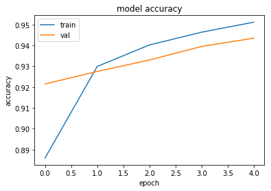
train Loss: 0.4130 Acc: 0.8860
60000
val Loss: 0.2651 Acc: 0.9215
10000
Epoch 1/4
----------
train Loss: 0.2437 Acc: 0.9299
60000
val Loss: 0.2316 Acc: 0.9275
10000
Epoch 2/4
----------
train Loss: 0.2067 Acc: 0.9402
60000
val Loss: 0.2121 Acc: 0.9330
10000
Epoch 3/4
----------
train Loss: 0.1851 Acc: 0.9464
60000
val Loss: 0.1969 Acc: 0.9395
10000
Epoch 4/4
----------
train Loss: 0.1699 Acc: 0.9512
60000
val Loss: 0.1891 Acc: 0.9435
10000
Training complete in 0m 50s
Best val Acc: 0.943500
plt.plot(history['train_acc'])
plt.plot(history['val_acc'])
plt.title('model accuracy')
plt.ylabel('accuracy')
plt.xlabel('epoch')
plt.legend(['train', 'val'], loc='upper left')
plt.show()
# summarize history for loss
plt.plot(history['train_loss'])
plt.plot(history['val_loss'])
plt.title('model loss')
plt.ylabel('loss')
plt.xlabel('epoch')
plt.legend(['train', 'val'], loc='upper left')
plt.show()

# initialize lists to monitor test loss and accuracy
test_loss = 0.0
class_correct = list(0. for i in range(10))
class_total = list(0. for i in range(10))

model.eval() # prep model for *evaluation*

for data, target in test_loader:
    # forward pass: compute predicted outputs by passing inputs to the model
    output = model(data)
    # calculate the loss
    loss = criterion(output, target)
    # update test loss
    test_loss += loss.item()*data.size(0)
    # convert output probabilities to predicted class
    _, pred = torch.max(output, 1)
    # compare predictions to true label
    correct = np.squeeze(pred.eq(target.data.view_as(pred)))
    # calculate test accuracy for each object class
    for i in range(batch_size):
        label = target.data[i]
        class_correct[label] += correct[i].item()
        class_total[label] += 1

# calculate and print avg test loss
test_loss = test_loss/len(test_loader.dataset)
print('Test Loss: {:.6f}\n'.format(test_loss))

for i in range(10):
    if class_total[i] > 0:
        print('Test Accuracy of %5s: %2d%% (%2d/%2d)' % (
            str(i), 100 * class_correct[i] / class_total[i],
            np.sum(class_correct[i]), np.sum(class_total[i])))
    else:
        print('Test Accuracy of %5s: N/A (no training examples)' % (classes[i]))

print('\nTest Accuracy (Overall): %2d%% (%2d/%2d)' % (
    100. * np.sum(class_correct) / np.sum(class_total),
    np.sum(class_correct), np.sum(class_total)))
Test Loss: 0.150191

Test Accuracy of     0: 97% (760/783)
Test Accuracy of     1: 98% (906/919)
Test Accuracy of     2: 92% (762/824)
Test Accuracy of     3: 89% (721/804)
Test Accuracy of     4: 94% (751/793)
Test Accuracy of     5: 97% (698/718)
Test Accuracy of     6: 93% (730/779)
Test Accuracy of     7: 94% (765/806)
Test Accuracy of     8: 90% (706/777)
Test Accuracy of     9: 92% (740/797)

Test Accuracy (Overall): 94% (7539/8000)
# obtain one batch of test images
dataiter = iter(test_loader)
images, labels = dataiter.next()

# get sample outputs
output = model(images)
# convert output probabilities to predicted class
_, preds = torch.max(output, 1)
# prep images for display
images = images.numpy()

# plot the images in the batch, along with predicted and true labels
fig = plt.figure(figsize=(25, 4))
for idx in np.arange(20):
    ax = fig.add_subplot(2, 20/2, idx+1, xticks=[], yticks=[])
    ax.imshow(np.squeeze(images[idx]), cmap='gray')
    ax.set_title("{} ({})".format(str(preds[idx].item()), str(labels[idx].item())),
                 color=("green" if preds[idx]==labels[idx] else "red"))

PyTorch Functional API
# [0-9] unique labels
num_classes = 10
epochs = 5
## Define the NN architecture
class Net(nn.Module):
    def __init__(self):
        super(Net, self).__init__()
        self.num_hidden1 = 16
        # linear layer (784 -> 1 hidden node)
        self.fc1 = nn.Linear(28 * 28, self.num_hidden1)
        self.output = nn.Linear(self.num_hidden1, num_classes)

    def forward(self, x):
        # flatten image input
        x = x.view(-1, 28 * 28)
        # 1 hidden layer, with relu activation function
        x = F.relu(self.fc1(x))
        x = F.log_softmax(self.output(x), dim=1)
        return x

# initialize the NN
model = Net()
model = model.to(device)
print(model)
Net(
  (fc1): Linear(in_features=784, out_features=16, bias=True)
  (output): Linear(in_features=16, out_features=10, bias=True)
)
# specify loss function
criterion = nn.NLLLoss()

# specify optimizer
optimizer = optim.Adam(model.parameters(), lr=1e-3)
def train_model(model, dataloaders, criterion, optimizer, num_epochs):
    since = time.time()

    history = dict()

    best_model_wts = copy.deepcopy(model.state_dict())
    best_acc = 0.0

    for epoch in range(num_epochs):
        print('Epoch {}/{}'.format(epoch, num_epochs - 1))
        print('-' * 10)

        # Each epoch has a training and validation phase
        for phase in ['train', 'val']:
            if phase == 'train':
                model.train()  # Set model to training mode
            else:
                model.eval()   # Set model to evaluate mode

            running_loss = 0.0
            running_corrects = 0

            # Iterate over data.
            for inputs, labels in dataloaders[phase]:
                inputs = inputs.to(device)
                labels = labels.to(device)

                # zero the parameter gradients
                optimizer.zero_grad()

                # forward
                # track history if only in train
                with torch.set_grad_enabled(phase == 'train'):
                    # Get model outputs and calculate loss

                    # backward + optimize only if in training phase
                    if phase == 'train':
                        outputs = model(inputs)
                        loss = criterion(outputs, labels)
                        loss.backward()
                        optimizer.step()

                    else:
                        outputs = model(inputs)
                        loss = criterion(outputs, labels)

                    _, preds = torch.max(outputs, 1)

                # statistics
                running_loss += loss.item() * inputs.size(0)
                running_corrects += torch.sum(preds == labels.data)

            epoch_loss = running_loss / (len(dataloaders[phase])*batch_size)
            epoch_acc = running_corrects.double() / (len(dataloaders[phase])*batch_size)

            print('{} Loss: {:.4f} Acc: {:.4f}'.format(phase, epoch_loss, epoch_acc))
            print (len(dataloaders[phase].dataset))

            # deep copy the model
            if phase == 'val' and epoch_acc > best_acc:
                best_acc = epoch_acc
                best_model_wts = copy.deepcopy(model.state_dict())

            if phase+'_acc' in history:
                # append the new number to the existing array at this slot
                history[phase+'_acc'].append(epoch_acc)
            else:
                # create a new array in this slot
                history[phase+'_acc'] = [epoch_acc]

            if phase+'_loss' in history:
                # append the new number to the existing array at this slot
                history[phase+'_loss'].append(epoch_loss)
            else:
                # create a new array in this slot
                history[phase+'_loss'] = [epoch_loss]

    time_elapsed = time.time() - since
    print('Training complete in {:.0f}m {:.0f}s'.format(time_elapsed // 60, time_elapsed % 60))
    print('Best val Acc: {:4f}'.format(best_acc))

    # load best model weights
    model.load_state_dict(best_model_wts)
    return model, history
model, history = train_model(model, dataloaders_dict, criterion, optimizer, epochs)
Epoch 0/4
----------
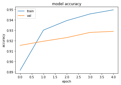
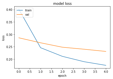
train Loss: 0.4015 Acc: 0.8915
60000
val Loss: 0.2860 Acc: 0.9155
10000
Epoch 1/4
----------
train Loss: 0.2460 Acc: 0.9302
60000
val Loss: 0.2658 Acc: 0.9195
10000
Epoch 2/4
----------
train Loss: 0.2112 Acc: 0.9394
60000
val Loss: 0.2480 Acc: 0.9230
10000
Epoch 3/4
----------
train Loss: 0.1895 Acc: 0.9458
60000
val Loss: 0.2399 Acc: 0.9280
10000
Epoch 4/4
----------
train Loss: 0.1748 Acc: 0.9497
60000
val Loss: 0.2310 Acc: 0.9290
10000
Training complete in 0m 52s
Best val Acc: 0.929000
plt.plot(history['train_acc'])
plt.plot(history['val_acc'])
plt.title('model accuracy')
plt.ylabel('accuracy')
plt.xlabel('epoch')
plt.legend(['train', 'val'], loc='upper left')
plt.show()
# summarize history for loss
plt.plot(history['train_loss'])
plt.plot(history['val_loss'])
plt.title('model loss')
plt.ylabel('loss')
plt.xlabel('epoch')
plt.legend(['train', 'val'], loc='upper left')
plt.show()
# initialize lists to monitor test loss and accuracy
test_loss = 0.0
class_correct = list(0. for i in range(10))
class_total = list(0. for i in range(10))

model.eval() # prep model for *evaluation*

for data, target in test_loader:
    # forward pass: compute predicted outputs by passing inputs to the model
    output = model(data)
    # calculate the loss
    loss = criterion(output, target)
    # update test loss
    test_loss += loss.item()*data.size(0)
    # convert output probabilities to predicted class
    _, pred = torch.max(output, 1)
    # compare predictions to true label
    correct = np.squeeze(pred.eq(target.data.view_as(pred)))
    # calculate test accuracy for each object class
    for i in range(batch_size):
        label = target.data[i]
        class_correct[label] += correct[i].item()
        class_total[label] += 1

# calculate and print avg test loss
test_loss = test_loss/len(test_loader.dataset)
print('Test Loss: {:.6f}\n'.format(test_loss))

for i in range(10):
    if class_total[i] > 0:
        print('Test Accuracy of %5s: %2d%% (%2d/%2d)' % (
            str(i), 100 * class_correct[i] / class_total[i],
            np.sum(class_correct[i]), np.sum(class_total[i])))
    else:
        print('Test Accuracy of %5s: N/A (no training examples)' % (classes[i]))

print('\nTest Accuracy (Overall): %2d%% (%2d/%2d)' % (
    100. * np.sum(class_correct) / np.sum(class_total),
    np.sum(class_correct), np.sum(class_total)))
Test Loss: 0.174892

Test Accuracy of     0: 96% (757/783)
Test Accuracy of     1: 99% (911/919)
Test Accuracy of     2: 90% (748/824)
Test Accuracy of     3: 89% (719/804)
Test Accuracy of     4: 94% (752/793)
Test Accuracy of     5: 97% (697/718)
Test Accuracy of     6: 94% (735/779)
Test Accuracy of     7: 91% (741/806)
Test Accuracy of     8: 84% (654/777)
Test Accuracy of     9: 94% (754/797)

Test Accuracy (Overall): 93% (7468/8000)
# obtain one batch of test images
dataiter = iter(test_loader)
images, labels = dataiter.next()

# get sample outputs
output = model(images)
# convert output probabilities to predicted class
_, preds = torch.max(output, 1)
# prep images for display
images = images.numpy()

# plot the images in the batch, along with predicted and true labels
fig = plt.figure(figsize=(25, 4))
for idx in np.arange(20):
    ax = fig.add_subplot(2, 20/2, idx+1, xticks=[], yticks=[])
    ax.imshow(np.squeeze(images[idx]), cmap='gray')
    ax.set_title("{} ({})".format(str(preds[idx].item()), str(labels[idx].item())),
                 color=("green" if preds[idx]==labels[idx] else "red"))

I-know-everything: Young Padwan, now you possess the Force of MLP. Now knock yourself and experiement with different number of layers. Also, watch for training and validation loss as hint if model is moving in right direction. There you will come across overfitting and underfiting. So, be sure to watch them and we will discuss about them in detail in next time where you will learn about Force of CNN and how they can further give us best model (Yes, better than MLP). Until next time, try different architectures, different datasets like cifar, cats-and-dogs, etc and keep researching and head onto Further Reading section.
Happy Learning!
Note: Caveats on terminology
Jedi Council of DeepMind - DeepMind
Force of NN- NN
Force of MLP - MLP
neuron - unit
jar jar backpropagation - backpropagation
non-linearity - activity function
(linear transform + non-linearity) - layer
Force of CNN - CNN
Further Reading
Chris Olah’s blog on backpropagation
Adam Geitgey’s Machine Learning is Fun! Part 1 and Part 2
Q.V. Le A Tutorial on Deep Learning Part 1: Nonlinear Classifiers and The Backpropagation Algorithm and Part 2: Autoencoders, Convolutional Neural Networks and Recurrent Neural Networks
CS231n: Backpropagation, Intuitions
CS231n: Minimal Neural Network Case Study
Yearning Book by Andrew Ng Chapters 1 to 3
CS231n Winter 2016 Lectures 1 to 7
Neural Networks and Deep Learning Chapters 1 and 2
Neural Networks, Manifolds, and Topology
The Matrix Calculus You Need For Deep Learning
An overview of gradient descent optimization algorithms
Single-Layer Neural Networks and Gradient Descent
The Unreasonable Reputation of Neural Networks
Back-propagation - Math Simplified
Footnotes and Credits
NOTE
Questions, comments, other feedback? E-mail the author