This post continues my series on distributed training techniques in PyTorch. In earlier posts, I implemented and profiled data parallelism and sharding strategies, and compared naive implementations with their optimized PyTorch counterparts.
In this installment, I revisit pipeline parallelism: how to implement it from scratch, how stage-to-stage communication works, and how different schedules show up in the profiler.
The core idea of pipeline parallelism is simple: split a sequential model across multiple GPUs. For a 24-layer model and 4 GPUs, a simple partition might look like this:
- GPU 0: Layers 1-6
- GPU 1: Layers 7-12
- GPU 2: Layers 13-18
- GPU 3: Layers 19-24
Each GPU becomes a stage in the pipeline and stores only its assigned portion of the model. During the forward pass, activations move from one stage to the next. During the backward pass, gradients flow in the reverse direction.
The idea is simple, but the implementation is not. The challenges include partitioning the model correctly and coordinating computation, activation transfer, gradient transfer, and optimizer updates across stages without deadlocks or excessive idle time.
Refresher on Pipeline Parallelism
Here’s the blog on pipeline parallelism.
In that post, I covered the main pipeline-parallel scheduling algorithms, the pipeline bubble problem, and the techniques used to reduce it. We started with the simplest schedule and progressively moved toward more optimized ones:
- Naive pipeline parallelism: Split the model across GPUs and process one batch at a time. Most GPUs spend a lot of time idle while waiting for upstream or downstream stages.
- GPipe: Split each batch into smaller micro-batches so multiple parts of the batch can be in flight at once, reducing idle time.
- 1F1B and Interleaved 1F1B: Reduce the bubble further by interleaving forward and backward work. This also lowers peak activation memory because activations can be freed earlier.
- Zero-Bubble: Pushes scheduling further by carefully reordering backward work to eliminate most of the remaining bubble.
- DualPipe: The schedule used in DeepSeek-V3, designed to overlap communication and computation more aggressively using a bidirectional schedule.
Setup
All the code snippets shown in this post are available at the github repo: llm-parallelism-pytorch.
Compared to the DDP and sharding experiments, the data pipeline and profiler setup remain mostly the same. The main changes are in how the model is partitioned and how the training step is executed on each stage.
- Model:
SmolLM2-360M-Instructmodel was used previously in DDP experiments. This model did not work as expected withtorch.distributed.pipeliningAPI to automatically split the model across GPUs. Instead, I use a DistilBERT modeldistilbert/distilbert-base-uncasedfor the classification task. The notes section of the project provides additional details on the exact errors encountered. - Data:
Yelp Reviewdataset - Data pipeline: The code for data pipeline that takes care of tokenization and batching to create training and validation data loaders is the same. The important change here is that the data is not sharded across ranks. In pipeline parallelism, every stage participates in the same training step, so the same batch must flow through all stages.
- PyTorch profiling: The profiler is used to capture memory usage, computation time, and communication time.
- Training loop: It consists of a training step with forward pass, calculating loss, backward pass and optimizer step. The implementation of training loop behaves differently depending on pipeline stage for the step.
The workflow for pipeline parallelism becomes:
- Modify the data pipeline so the same batch is visible to all pipeline stages
- Split the model into stage-local modules
- Create a stage-local optimizer for the parameters owned by that stage
- Run a training loop where the forward and backward logic depends on the stage index
Forward pass
The forward pass behaves differently depending on which stage is executing it:
- Stage 0 receives the input batch, runs its local chunk of the model, and sends the resulting activations to the next stage.
- Intermediate stages receive activations from the previous stage, run their local chunk, and forward the new activations onward.
- The final stage receives activations from the previous stage, runs the last chunk of the model, and computes the loss.
Backward pass
The backward pass flows in the reverse direction:
- The last stage starts backpropagation from the loss and sends activation gradients to the previous stage.
- Intermediate stages receive gradients from the next stage, backpropagate through their local chunk, and send input gradients to the previous stage.
- Stage 0 receives gradients from stage 1 and completes the backward pass for the first chunk of the model.
Optimizer step
Because each stage owns a disjoint subset of the parameters, each stage can apply its optimizer step independently after the backward pass completes.

Here is what the flow for forward and backward pass looks like for splitting 6 layers across 3 GPUs. It saves activations across the pipeline stages which are reused for calculating backward gradients.
Hypothesis
Before implementing and profiling the schedules, it is useful to write down the patterns we expect to see.
- Naive pipeline: We should see large, clearly separated forward, backward, and optimizer regions for each stage, with substantial idle gaps between them.
- GPipe: The same work should now be broken into smaller chunks because the batch is split into multiple micro-batches. This should reduce the visible pipeline bubble.
- 1F1B: We should see forward and backward work interleaved after the warmup phase. We should also expect lower peak activation memory than GPipe or naive scheduling, because activations do not need to stay alive for as long.
Setting up pipeline parallelism
Two things are essential for pipeline parallelism setup
- Splitting the model
- Establishing the peer-to-peer communication between neighboring GPUs
Splitting the model
How you split the model matters. A poor split can create load imbalance across stages, increase memory pressure, and introduce unnecessary stalls.
The split_model_for_scratch function builds the stage-local module for each rank. The model is partitioned using the following rules:
- The embedding layers belong to the first stage
- The final classification layers belong to the last stage
- The transformer blocks in between are split as evenly as possible across the remaining stages
This strategy works well for encoder-style models such as DistilBERT, where the repeated transformer blocks dominate most of the compute.
Implementation
def get_pp_layers(model: torch.nn.Module) -> nn.ModuleList:
    """Return the encoder layers used for PP splitting."""
    if not hasattr(model, "distilbert") or not hasattr(model.distilbert, "transformer"):
        raise ValueError("Expected DistilBERT backbone for pipeline parallelism.")
    return model.distilbert.transformer.layer

def stage_bounds(n_layers: int, num_stages: int, rank: int) -> tuple[int, int]:
    # even split with remainder on early ranks
    base = n_layers // num_stages
    rem = n_layers % num_stages
    start = rank * base + min(rank, rem)
    end = start + base + int(rank < rem)
    return start, end

def build_stage_module(model: torch.nn.Module, num_stages: int, rank: int):
    """Build one DistilBERT stage module for either scratch or PyTorch PP."""
    layers = get_pp_layers(model)
    n_layers = len(layers)
    start, end = stage_bounds(n_layers, num_stages, rank)
    is_first = rank == 0
    is_last = rank == num_stages - 1

    class ScratchStageModule(nn.Module):
        def __init__(self):
            super().__init__()
            self.embeddings = model.distilbert.embeddings if is_first else None
            self.layers = nn.ModuleList(layers[start:end])
            self.pre_classifier = getattr(model, "pre_classifier", None) if is_last else None
            self.dropout = getattr(model, "dropout", None) if is_last else None
            self.classifier = getattr(model, "classifier", None) if is_last else None
            self._attention_mask_chunks: tuple[torch.Tensor, ...] = ()
            self._next_mask_idx = 0

        def prepare_microbatch_attention_mask(
            self, attention_mask: torch.Tensor, num_microbatches: int
        ) -> None:
            """Cache the local attention-mask chunks for PyTorch PP schedules."""
            device = next(self.parameters()).device
            self._attention_mask_chunks = tuple(
                chunk.to(device, non_blocking=True)
                for chunk in attention_mask.chunk(num_microbatches, dim=0)
            )
            self._next_mask_idx = 0

        def _resolve_attention_mask(
            self, hidden_states: torch.Tensor, attention_mask: torch.Tensor | None
        ) -> torch.Tensor:
            """Use explicit mask when present, otherwise consume the next cached chunk."""
            if attention_mask is None:
                if self._next_mask_idx < len(self._attention_mask_chunks):
                    attention_mask = self._attention_mask_chunks[self._next_mask_idx]
                    self._next_mask_idx += 1
                else:
                    attention_mask = torch.ones(
                        hidden_states.shape[:2], device=hidden_states.device, dtype=torch.bool
                    )
            return attention_mask

        def forward(self, x, attention_mask=None):
            """Run this stage shard.

            Args:
                x: First stage expects token ids [B, S]; other stages expect hidden states [B, S, H].
                attention_mask: Optional mask [B, S] propagated across stages.

            Returns:
                Hidden states [B, S, H] for non-last stages, or classifier output on last stage.
            """
            # Stage 0: token ids [B, S] -> embeddings [B, S, H].
            # Other stages: x is already hidden states [B, S, H].
            hidden_states = self.embeddings(x) if self.embeddings is not None else x
            attention_mask = self._resolve_attention_mask(hidden_states, attention_mask)
            attention_mask_2d = attention_mask.to(
                hidden_states.device, dtype=torch.bool, non_blocking=True
            )
            attention_mask = attention_mask_2d
            if model.config._attn_implementation == "sdpa":
                attention_mask = _prepare_4d_attention_mask_for_sdpa(
                    attention_mask,
                    hidden_states.dtype,
                    tgt_len=hidden_states.shape[1],
                )

            for layer in self.layers:
                # Encoder block preserves hidden shape: [B, S, H] -> [B, S, H].
                out = layer(hidden_states, attn_mask=attention_mask)
                hidden_states = out[0] if isinstance(out, tuple) else out

            if self.classifier is not None:
                pooled_output = hidden_states[:, 0]
                if self.pre_classifier is not None:
                    pooled_output = self.pre_classifier(pooled_output)
                    pooled_output = F.relu(pooled_output)
                if self.dropout is not None:
                    pooled_output = self.dropout(pooled_output)
                return self.classifier(pooled_output)
            # Scratch stages send hidden states [B, S, H] only.
            return hidden_states

    return ScratchStageModule()

def split_model_for_scratch(model: torch.nn.Module, num_stages: int, rank: int):
    """Build rank-local module shard for scratch PP."""
    return build_stage_module(model, num_stages, rank)
Initializing P2P communication
Pipeline parallelism relies on point-to-point communication between neighboring stages. That means each stage must be able to safely send activations forward and send gradients backward without deadlocking.
In practice, the first communication between ranks can trigger lazy NCCL initialization, so I use the same technique used in PyTorch to pre-warm the communication paths using a dummy exchange.
The _initialize_p2p function in BasePipeline performs a small dummy send/receive exchange in both directions and in a fixed order. This pre-warms NCCL communication paths and makes the real training step less likely to hit lazy-init stalls or deadlocks.
The batch_isend_irecv function from PyTorch lets us batch point-to-point sends and receives in a fixed order. The API itself is asynchronous, but in this warmup path I explicitly wait for completion so the communication channels are initialized deterministically before real training begins.
Implementation
class BasePipeline(ABC):
    ...

    def _initialize_p2p(self) -> None:
        """Pre-warm NCCL P2P channels with dummy tensors to avoid lazy-init deadlocks."""
        if self._p2p_initialized:
            return
        dummy = torch.zeros(1, device=self.device)
        ops: list[dist.P2POp] = []
        # Forward direction: recv from prev, send to next
        if not self.is_first:
            ops.append(dist.P2POp(dist.irecv, dummy.clone(), self.stage - 1, self.pp_group))
        if not self.is_last:
            ops.append(dist.P2POp(dist.isend, dummy.clone(), self.stage + 1, self.pp_group))
        # Backward direction: recv from next, send to prev
        if not self.is_last:
            ops.append(dist.P2POp(dist.irecv, dummy.clone(), self.stage + 1, self.pp_group))
        if not self.is_first:
            ops.append(dist.P2POp(dist.isend, dummy.clone(), self.stage - 1, self.pp_group))
        if ops:
            reqs = dist.batch_isend_irecv(ops)
            for r in reqs:
                r.wait()
        self._p2p_initialized = True
Naive pipeline
The naive pipeline schedule is the simplest place to start.
We split the model across stages, process one full batch through the pipeline, run the backward pass in reverse, and finally apply the optimizer step. This introduces idle time where one GPU is waiting for input from previous stage, also called the pipeline bubbles.
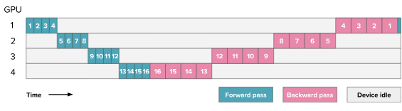
HuggingFace blog. Here the numbers indicate the layers processed for a single batch.
Using the model split described in Splitting the model, each GPU owns one stage-local chunk of the network. We can now implement the naive schedule.
The schedule consists of the following steps:
- Initializing peer-to-peer communication
Before starting the training step, we need to make sure communication between neighboring GPUs is ready and follows a consistent order. Otherwise, it is easy to end up in a deadlock. We use the _initialize_p2p function to warm up the communication paths with dummy tensors.
- Forward pass
The forward pass behaves differently depending on which stage is executing it:
- First stage: Moves the input batch to the local device, runs the local chunk of the model, saves the output for backpropagation, and sends the activations to the next stage.
- Intermediate stages: Receive activations from the previous stage, run the local chunk, save the output, and forward the new activations to the next stage.
- Final stage: Receives activations from the previous stage, runs the final chunk, and computes the loss.
One subtle but important detail is the explicit detach().requires_grad_() on received activations. Point-to-point communication does not preserve the autograd graph across ranks, so each receiving stage has to treat incoming activations as leaf tensors and manually send their gradients back during the backward pass.
Implementation
def forward_step() -> None:
    """Run stage-local forward for the single microbatch."""
    # First stage, we run the forward pass on the input batch
    # and send the activations to the next stage.
    if self.is_first:
        input_ids = batch["input_ids"].to(self.device, non_blocking=True)
        attention_mask = batch["attention_mask"].to(self.device, non_blocking=True)
        out = self.stage_module(input_ids, attention_mask)
        self._saved_output = out
        self._send(out, dst=self.stage + 1)
    # Last stage, we receive the activations from the previous stage,
    # run the forward pass to get logits and calculate the loss with the labels.
    elif self.is_last:
        buf = self._recv(buf=self.activation_recv_buffer, src=self.stage - 1)
        # Explicitly marking require grads as cross rank communication breaks autograd history
        buf = buf.detach()
        buf.requires_grad_()
        self._saved_input = buf
        attention_mask = batch["attention_mask"].to(self.device, non_blocking=True)
        logits = self.stage_module(buf, attention_mask=attention_mask)
        labels = batch["labels"].to(self.device, non_blocking=True)
        self.loss = self.loss_fn(logits, labels, attention_mask=attention_mask)
    # Intermediate stage, we receive the activations from the previous stage,
    # run the forward pass, and send the activations to the next stage.
    else:
        buf = self._recv(buf=self.activation_recv_buffer, src=self.stage - 1)
        # Explicitly marking require grads as cross rank communication breaks autograd history
        buf = buf.detach()
        buf.requires_grad_()
        self._saved_input = buf
        attention_mask = batch["attention_mask"].to(self.device, non_blocking=True)
        out = self.stage_module(buf, attention_mask=attention_mask)
        self._saved_output = out
        self._send(out, dst=self.stage + 1)
- Backward pass
The backward pass runs in the reverse direction, starting from the last stage.
- Last stage: Calls
loss.backward()to begin backpropagation, then sends the gradient of its input activations to the previous stage. - Intermediate stages: Receive gradients from the next stage, backpropagate through their saved output, and send the resulting input gradients to the previous stage.
- First stage: Receives the gradient from stage 1 and backpropagates through its saved output.
Implementation
def backward_step() -> None:
    """Run stage-local backward for the single microbatch."""
    # Last stage starts the backward pass by calling `loss.backward()`,
    # then sends the input gradient to the previous stage.
    if self.is_last:
        self.loss.backward()
        grad_to_send = self._saved_input.grad
        self._send(grad_to_send, dst=self.stage - 1)
    # Intermediate stage receives the input gradient from the next stage,
    # runs backward on the intermediate activation,
    # and sends the gradient of the input activation to the previous stage.
    elif not self.is_first:
        grad_to_recv = self._recv(buf=self.gradient_recv_buffer, src=self.stage + 1)
        self._saved_output.backward(grad_to_recv)
        grad_to_send = self._saved_input.grad
        self._send(grad_to_send, dst=self.stage - 1)
    # First stage receives the input gradient from the next stage
    # and runs backward on the input activation.
    else:
        grad_to_recv = self._recv(buf=self.gradient_recv_buffer, src=self.stage + 1)
        # For stage 0, saved activation is the output we sent onward.
        self._saved_output.backward(grad_to_recv)
- Training step
For a single batch, the stage-local training step is straightforward:
- initialize communication if needed
- zero the gradients for the local stage
- run forward
- run backward
- apply the stage-local optimizer step
Each stage only updates the parameters it owns.
Implementation
def run_batch(self, batch):
    assert self.num_microbatches == 1, "NaivePipeline only supports num_microbatches=1"

    self._initialize_p2p()
    self.stage_opt.zero_grad(set_to_none=True)
    self.loss = None
    # Forward pass and calculate loss
    with torch.profiler.record_function("pp.forward"):
        forward_step()

    # Backward pass
    with torch.profiler.record_function("pp.backward"):
        backward_step()

    # Optimizer step for particular stage
    with torch.profiler.record_function("pp.optimizer_step"):
        self.stage_opt.step()

    # Free the space taken by saved activation
    self._saved_input = None
    self._saved_output = None
    # Calculate final loss
    final_loss = self.loss.item() if self.is_last and self.loss is not None else None
    self.loss = None
    return final_loss
Result
In the profiler, the naive schedule should show large contiguous blocks of forward work followed by backward work, with noticeable idle gaps on most stages. The first stage becomes idle after sending activations forward, while the last stage remains idle until enough upstream work has completed for it to begin. These idle regions are the pipeline bubble in its most obvious form.
That is exactly what the trace shows. The CPU-side pp.forward, pp.backward, and pp.optimizer_step spans are easy to distinguish, while the GPU stream view is dominated by long NCCL P2P regions and obvious idle gaps between stages. The middle stage also has the heaviest communication burden because it talks to both neighbors in both directions.

The summary metrics line up with that trace shape. Naive PP has the largest communication overhead in this experiment at roughly 68% of kernel time, and its average peak allocated memory is about 1.25 GB. So the schedule is simple and correct, but the bubble is large and utilization is poor.
Profiling
GPipe pipeline
GPipe improves GPU utilization by splitting a batch into smaller micro-batches. Instead of waiting for a full batch to move stage by stage, the pipeline can keep multiple micro-batches in flight at the same time, which reduces idle time and shrinks the pipeline bubble.
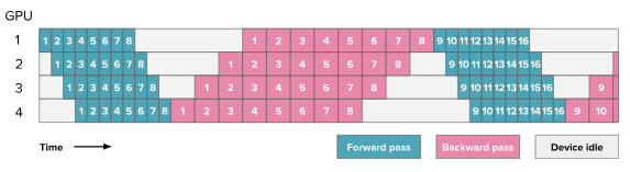
HuggingFace blog. Here the numbers indicate the micro-batches.
Using the model split described in Splitting the model, each GPU owns one stage-local chunk of the network. We can now implement the GPipe schedule.
The schedule consists of the following steps:
- Initializing peer-to-peer communication
The same warmup process used in the naive pipeline is reused here to initialize communication across neighboring GPUs.
- Chunk batch into microbatches
A full batch is split along the batch dimension into num_microbatches smaller pieces:
chunks = {k: v.chunk(self.num_microbatches, dim=0) for k, v in batch.items()}
micro_batches = [{k: chunks[k][i] for k in chunks} for i in range(self.num_microbatches)]
This is the key idea behind GPipe. More micro-batches usually reduce the pipeline bubble, although they also increase scheduling overhead.
- Forward pass
The forward-pass logic is the same as in the naive pipeline, but it is now executed once per micro-batch.
The main difference in the implementation compared to naive implementation is we use a list and keep track of saved input, output activation and loss for each micro-batch at each stage of the pipeline indexed by micro_batch_idx.
Implementation
def forward_micro(micro_batch_idx: int) -> None:
    """Run one microbatch forward for this stage."""
    micro_batch = micro_batches[micro_batch_idx]
    # First stage, we run the forward pass on the input batch
    # and send the activations to the next stage.
    if self.is_first:
        input_ids = micro_batch["input_ids"].to(self.device, non_blocking=True)
        attention_mask = micro_batch["attention_mask"].to(self.device, non_blocking=True)
        out = self.stage_module(input_ids, attention_mask)
        self._saved_output[micro_batch_idx] = out
        self._send(out, dst=self.stage + 1)
    # Last stage, we receive the activations from the previous stage,
    # run the forward pass to get logits and calculate the loss with the labels.
    elif self.is_last:
        buf = self._recv(
            buf=self.activation_recv_buffers[micro_batch_idx], src=self.stage - 1
        )
        buf = buf.detach()
        buf.requires_grad_()
        self._saved_input[micro_batch_idx] = buf
        attention_mask = micro_batch["attention_mask"].to(self.device, non_blocking=True)
        logits = self.stage_module(buf, attention_mask=attention_mask)
        labels = micro_batch["labels"].to(self.device, non_blocking=True)
        self.losses[micro_batch_idx] = self.loss_fn(
            logits, labels, attention_mask=attention_mask
        )
    # Intermediate stage, we receive the activations from the previous stage,
    # run the forward pass, and send the activations to the next stage.
    else:
        buf = self._recv(
            buf=self.activation_recv_buffers[micro_batch_idx], src=self.stage - 1
        )
        buf = buf.detach()
        buf.requires_grad_()
        self._saved_input[micro_batch_idx] = buf
        attention_mask = micro_batch["attention_mask"].to(self.device, non_blocking=True)
        out = self.stage_module(buf, attention_mask=attention_mask)
        self._saved_output[micro_batch_idx] = out
        self._send(out, dst=self.stage + 1)
- Backward pass
After all micro-batches complete the forward phase, the backward phase runs in reverse micro-batch order. This is the classic all-forward, all-backward schedule used by GPipe.
As in the forward phase, each stage keeps separate gradient buffers for each micro-batch.
Implementation
def backward_micro(micro_batch_idx: int) -> None:
    """Run one microbatch backward for this stage."""
    # Last stage starts the backward pass by calling `loss.backward()`,
    # then sends the input gradient to the previous stage.
    if self.is_last:
        # Match full-batch mean-loss scaling across microbatches.
        (self.losses[micro_batch_idx] / self.num_microbatches).backward()
        grad_to_send = self._saved_input[micro_batch_idx].grad
        self._send(grad_to_send, dst=self.stage - 1)
    # Intermediate stage receives the input gradient from the next stage,
    # runs backward on the intermediate activation,
    # and sends the gradient of the input activation to the previous stage.
    elif not self.is_first:
        grad_to_recv = self._recv(
            buf=self.gradient_recv_buffers[micro_batch_idx], src=self.stage + 1
        )
        self._saved_output[micro_batch_idx].backward(grad_to_recv)
        grad_to_send = self._saved_input[micro_batch_idx].grad
        self._send(grad_to_send, dst=self.stage - 1)
    # First stage receives the input gradient from the next stage
    # and runs backward on the input activation.
    else:
        grad_to_recv = self._recv(
            buf=self.gradient_recv_buffers[micro_batch_idx], src=self.stage + 1
        )
        # For stage 0, saved activation is the output we sent onward.
        self._saved_output[micro_batch_idx].backward(grad_to_recv)
- Training step
For each batch, we first split the batch into micro-batches. We then run the forward pass for all micro-batches, followed by the backward pass for all micro-batches in reverse order, and finally apply the optimizer step.
Implementation
def run_batch(...):
    assert self.num_microbatches > 1, "GPipe requires num_microbatches>1"

    self._initialize_p2p()
    self.stage_opt.zero_grad(set_to_none=True)

    ...

    # Chunk to create microbatches
    chunks = {k: v.chunk(self.num_microbatches, dim=0) for k, v in batch.items()}
    micro_batches = [{k: chunks[k][i] for k in chunks} for i in range(self.num_microbatches)]

    ...

    # Forward pass and calculate loss
    with torch.profiler.record_function("pp.forward"):
        for micro_batch_idx in range(self.num_microbatches):
            forward_micro(micro_batch_idx)

    # Backward pass in reverse
    with torch.profiler.record_function("pp.backward"):
        for micro_batch_idx in range(self.num_microbatches - 1, -1, -1):
            backward_micro(micro_batch_idx)

    # Optimizer step for particular stage
    with torch.profiler.record_function("pp.optimizer_step"):
        self.stage_opt.step()
    # Free the activation memory
    self._saved_input = [None] * self.num_microbatches
    self._saved_output = [None] * self.num_microbatches
    final_loss = None
    if self.is_last:
        loss_vals = [loss.detach() for loss in self.losses if loss is not None]
        final_loss = torch.stack(loss_vals).mean().item() if loss_vals else None
    self.losses = [None] * self.num_microbatches
    return final_loss
One important tradeoff in GPipe is memory. Although micro-batching improves utilization, the all-forward, all-backward schedule means activations from earlier micro-batches must remain alive until backward begins. As a result, GPipe can still have high activation memory overhead.
Result
In the profiler, GPipe should break the large forward and backward regions of the naive schedule into smaller per-microbatch chunks. The bubble does not disappear completely, but it becomes smaller because multiple micro-batches can occupy different stages simultaneously.
The trace behaves that way. Instead of one large forward block and one large backward block, each stage now processes a stream of micro-batch-sized chunks. The last stage still sits idle during the fill phase, so the bubble does not disappear, but the timeline is much denser than in the naive schedule.

Profiling also shows the main GPipe tradeoff clearly. Among the scratch implementations it has the best compute utilization and the lowest total P2P kernel time, but it still keeps more activations alive than 1F1B because backward begins only after all forward micro-batches finish.
Profiling
1F1B pipeline
1F1B (one-forward-one-backward) improves on GPipe by interleaving forward and backward work once the pipeline is full.
The main benefit is lower peak activation memory: instead of storing activations for all micro-batches until the backward phase begins, each stage can start backpropagating earlier and free older activations sooner.
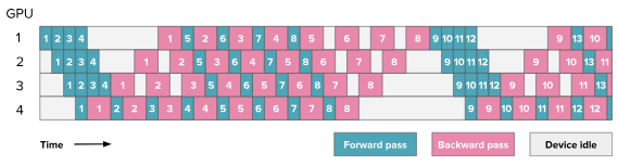
HuggingFace blog
Using the model split described in Splitting the model, each GPU owns one stage-local chunk of the network. We can now implement the 1F1B schedule.
Unlike the naive and GPipe schedules, 1F1B is no longer just “run forward” and then “run backward”. Each stage now follows a local schedule with three phases:
- Warmup: forward-only steps to fill the pipeline
- Steady state: alternate one backward step and one forward step
- Drain: backward-only steps to flush the remaining work
The number of warmup steps depends on the stage:
warmup_steps = min(num_stages - stage - 1, num_microbatches)
So for a 4-stage pipeline:
- stage 0 performs the most warmup steps
- intermediate stages perform fewer
- the last stage performs no warmup, because it can start backward as soon as it finishes its first forward
This staggered setup is what lets later stages begin backpropagation while earlier stages are still processing newer micro-batches.
The schedule consists of the following steps:
- Initializing peer-to-peer communication
The same warmup process used in the naive and GPipe pipeline is reused here to initialize communication across neighboring GPUs.
- Chunk batch into microbatches
As in GPipe, the batch is split along the batch dimension into smaller micro-batches:
chunks = {k: v.chunk(self.num_microbatches, dim=0) for k, v in batch.items()}
micro_batches = [{k: chunks[k][i] for k in chunks} for i in range(self.num_microbatches)]
- Forward pass
The forward computation for one micro-batch is similar to the earlier schedules:
- First stage: takes token IDs as input, runs the local module, and stores the output
- Intermediate stages: receive activations from the previous stage, mark them as gradient-carrying leaf tensors, run the local module, and store both input and output
- Last stage: receives activations, runs the local module, and computes the loss for that micro-batch
The forward computation itself is essentially the same as in GPipe. The main difference from GPipe is not the forward computation itself, but when it happens relative to backward. In 1F1B, forward execution is interleaved with backward execution after the warmup phase.
Implementation
def _forward_compute(self, micro_batch_idx: int, micro_batches: list[dict]) -> None:
    """Run forward computation for one microbatch (no P2P)."""
    micro_batch = micro_batches[micro_batch_idx]

    if self.is_first:
        input_ids = micro_batch["input_ids"].to(self.device, non_blocking=True)
        attention_mask = micro_batch["attention_mask"].to(self.device, non_blocking=True)
        out = self.stage_module(input_ids, attention_mask=attention_mask)
        self._saved_output[micro_batch_idx] = out
    else:
        buf = self.activation_recv_buffers[micro_batch_idx]
        buf = buf.detach()
        buf.requires_grad_()
        self._saved_input[micro_batch_idx] = buf

        attention_mask = micro_batch["attention_mask"].to(self.device, non_blocking=True)
        out = self.stage_module(buf, attention_mask=attention_mask)

        if self.is_last:
            labels = micro_batch["labels"].to(self.device, non_blocking=True)
            self.losses[micro_batch_idx] = self.loss_fn(
                out, labels, attention_mask=attention_mask
            )
        else:
            self._saved_output[micro_batch_idx] = out
- Backward pass
The backward computation is also stage-local:
- Last stage: starts from the micro-batch loss
- Intermediate stages: receive gradients from the next stage and backpropagate through their saved output
- First stage: backpropagates using the gradient received from stage 1
As with GPipe, gradients must be communicated explicitly across stages because autograd does not span point-to-point communication boundaries.
Implementation
def _backward_compute(self, micro_batch_idx: int) -> None:
    """Run backward computation for one microbatch (no P2P)."""
    if self.is_last:
        (self.losses[micro_batch_idx] / self.num_microbatches).backward()
    else:
        grad = self.gradient_recv_buffers[micro_batch_idx]
        self._saved_output[micro_batch_idx].backward(grad)
- Training step
The full 1F1B training step is where the schedule becomes interesting.
Warmup phase
In the warmup phase, each stage performs forward-only work. The goal is to fill the pipeline with enough micro-batches so that backward work can begin without starving downstream stages.
Earlier stages have more warmup steps because they are farther from the loss. Later stages have fewer, and the last stage has none.
Steady-state phase
Once the pipeline is full, each stage alternates between:
- one backward step for an older micro-batch
- one forward step for a newer micro-batch
This is the “1F1B” part of the schedule.
A useful detail in this implementation is that communication is batched using dist.batch_isend_irecv. Instead of issuing sends and receives independently, complementary operations are fused together:
- forward send + backward receive
- backward send + forward receive
This mirrors PyTorch’s Schedule1F1B behavior and helps avoid deadlocks while keeping communication order consistent across stages.
Drain phase
After all forward work has been launched, the remaining micro-batches still need to finish backpropagation. The drain phase runs the remaining backward-only steps until the pipeline is empty.
Implementation
def run_batch(self, batch):
    """Run one non-interleaved 1F1B step over `num_microbatches`."""
    assert self.num_microbatches > 1, "1F1B requires num_microbatches>1"

    self._initialize_p2p()
    self.stage_opt.zero_grad(set_to_none=True)

    self._saved_input = [None] * self.num_microbatches
    self._saved_output = [None] * self.num_microbatches

    assert batch["input_ids"].size(0) % self.num_microbatches == 0, (
        "Batch size must be divisible by num_microbatches"
    )
    chunks = {k: v.chunk(self.num_microbatches, dim=0) for k, v in batch.items()}
    micro_batches = [{k: chunks[k][i] for k in chunks} for i in range(self.num_microbatches)]

    self.losses = [None] * self.num_microbatches

    warmup_steps = min(self.num_stages - self.stage - 1, self.num_microbatches)
    steady_steps = self.num_microbatches - warmup_steps
    fwd_idx = 0
    bwd_idx = 0

    # Warmup: forward-only
    fwd_sends: list[dist.P2POp] = []
    with torch.profiler.record_function("pp.forward_warmup"):
        for _ in range(warmup_steps):
            fwd_recvs = self._fwd_recv_ops(fwd_idx)
            self._exec_p2p(fwd_recvs)

            self._forward_compute(fwd_idx, micro_batches)

            fwd_sends = self._fwd_send_ops(fwd_idx)
            if fwd_idx != warmup_steps - 1:
                self._exec_p2p(fwd_sends)
                fwd_sends = []

            fwd_idx += 1

    # Last stage needs its first forward before steady-state backward can begin
    if warmup_steps == 0:
        fwd_recvs = self._fwd_recv_ops(fwd_idx)
        self._exec_p2p(fwd_recvs)
        self._forward_compute(fwd_idx, micro_batches)
        fwd_sends = self._fwd_send_ops(fwd_idx)
        fwd_idx += 1

    # Steady state: alternate one backward and one forward
    with torch.profiler.record_function("pp.1f1b_steady"):
        for _ in range(steady_steps):
            bwd_recvs = self._bwd_recv_ops(bwd_idx)
            self._exec_p2p(fwd_sends + bwd_recvs)

            self._backward_compute(bwd_idx)
            bwd_sends = self._bwd_send_ops(bwd_idx)
            bwd_idx += 1

            if fwd_idx < self.num_microbatches:
                fwd_recvs = self._fwd_recv_ops(fwd_idx)
                self._exec_p2p(bwd_sends + fwd_recvs)

                self._forward_compute(fwd_idx, micro_batches)
                fwd_sends = self._fwd_send_ops(fwd_idx)
                fwd_idx += 1
            else:
                self._exec_p2p(bwd_sends)
                fwd_sends = []

    # Drain: backward-only
    with torch.profiler.record_function("pp.backward_drain"):
        for _ in range(warmup_steps):
            bwd_recvs = self._bwd_recv_ops(bwd_idx)
            self._exec_p2p(fwd_sends + bwd_recvs)
            fwd_sends = []

            self._backward_compute(bwd_idx)
            bwd_sends = self._bwd_send_ops(bwd_idx)
            self._exec_p2p(bwd_sends)
            bwd_idx += 1

    with torch.profiler.record_function("pp.optimizer_step"):
        self.stage_opt.step()

    final_loss = None
    if self.is_last:
        loss_vals = [loss.detach() for loss in self.losses if loss is not None]
        final_loss = torch.stack(loss_vals).mean().item() if loss_vals else None

    self._saved_input = [None] * self.num_microbatches
    self._saved_output = [None] * self.num_microbatches
    self.losses = [None] * self.num_microbatches
    return final_loss
Result
In the profiler, 1F1B should look different from GPipe in two ways:
- forward and backward work should appear interleaved during the steady-state region
- peak memory usage should be lower because activations are freed earlier
The pipeline bubble is also smaller than in the naive schedule. Compared to GPipe, the main visible difference is not just utilization, but the much more fine-grained alternation of forward and backward work in the trace.
The traces confirm the memory part of that hypothesis much more strongly than the throughput part. The warmup, steady-state, and drain phases are visible in the CPU spans, and peak allocated memory drops sharply relative to GPipe because older activations can be released earlier.

In the scratch implementation, average peak allocated memory falls to about 596 MB, roughly half of scratch GPipe.
At the same time, the scratch 1F1B trace still spends a large fraction of time stalled in communication. The schedule is more memory-efficient, but the explicit batch_isend_irecv(...).wait() pattern leaves little compute/communication overlap.
Profiling
PyTorch pipeline parallelism
So far, the focus has been on implementing pipeline parallelism from scratch. That helps in understanding exactly how activations, gradients, and schedules flow across stages.
PyTorch also provides a higher-level pipeline API through torch.distributed.pipelining. In principle, this lets us reuse the same model split while delegating the scheduling logic to PyTorch.
For this setup, I do not use the automatic pipeline(...) frontend. That API traces the full graph and tries to infer stage boundaries automatically. On this DistilBERT classifier path, it fails during backward setup with the error:
Backward of skip connections not supported yet
To avoid that issue, I manually construct each PipelineStage.
def build_pytorch_stage(model: torch.nn.Module, rank: int, device: torch.device, pp_group):
    """Build a manual PipelineStage for PyTorch PP.

    The automatic `pipeline(...)` frontend traces the full graph and infers
    stage boundaries. On this DistilBERT classifier path it fails during
    backward setup with `Backward of skip connections not supported yet`.

    Manual stage construction avoids that frontend and lets us keep the stage
    split explicit while delegating the execution schedule to PyTorch.
    """
    stage_module = build_stage_module(model, dist.get_world_size(pp_group), rank)
    stage_module = stage_module.to(device)
    stage = PipelineStage(stage_module, rank, dist.get_world_size(pp_group), device, group=pp_group)
    return stage
The key idea here is that the stage split remains manual and the execution schedule is handed over to PyTorch.
GPipe pipeline
Once the stage is built, using PyTorch’s GPipe schedule is quite compact. PyTorch takes care of the micro-batch scheduling, communication ordering, and execution flow.
if args.pp_choice == "pytorch_GPipe_pp":
    stage = build_pytorch_stage(model, pp_rank, device, pp_group)
    schedule = ScheduleGPipe(stage, n_microbatches=NUM_MICROBATCHES, loss_fn=pp_loss_fn)
    optimizer = torch.optim.AdamW(stage.submod.parameters(), lr=5e-5)
    engine = PytorchPPEngine(
        schedule=schedule,
        optimizer=optimizer,
        device=device,
        model_for_memory=stage.submod,
        pp_group=pp_group,
    )
Results
Compared to the scratch GPipe implementation, the PyTorch trace is noticeably tighter.

The GPU streams spend a larger fraction of time in compute kernels, communication overhead is lower, and the trace analysis shows meaningful compute and communication overlap. In this setup, PyTorch GPipe reaches roughly 59% compute utilization with about 15% communication overlap.
The tradeoff is memory. PyTorch GPipe has the highest peak memory footprint of all schedules in this experiment, close to 2.0 GB on average across ranks. So it is a useful reference for utilization, but not for activation memory.
Profiling
1F1B pipeline
Switching from GPipe to 1F1B is similarly straightforward:
elif args.pp_choice == "pytorch_1f1b_pp":
    stage = build_pytorch_stage(model, pp_rank, device, pp_group)
    schedule = Schedule1F1B(stage, n_microbatches=NUM_MICROBATCHES, loss_fn=pp_loss_fn)
    optimizer = torch.optim.AdamW(stage.submod.parameters(), lr=5e-5)
    engine = PytorchPPEngine(
        schedule=schedule,
        optimizer=optimizer,
        device=device,
        model_for_memory=stage.submod,
        pp_group=pp_group,
    )
Results
PyTorch 1F1B keeps most of PyTorch GPipe’s utilization advantage while recovering a large chunk of the memory lost to the all-forward, all-backward schedule.

Average peak allocated memory drops from about 1.99 GB in PyTorch GPipe to about 900 MB here, while compute utilization stays close to 59%.
The CPU pp.* spans show the schedule directly, while the GPU streams mostly show compute kernels and NCCL send/recv kernels. The last stage often has the clearest pp.forward annotation on stream views because that is where the terminal forward work and loss computation are launched.
Profiling
Profiling insights
The profiling takeaways for each of the implementations are:
- Naive PP makes the bubble easiest to see, but it also spends the largest fraction of time stalled on communication.
- Scratch GPipe improves utilization the most among the handwritten schedules, but it keeps activation memory high because backward starts late.
- Scratch 1F1B delivers the intended memory reduction, but blocking P2P waits prevent that from turning into better throughput here.
- PyTorch schedules are consistently more efficient in the trace, with much better compute utilization and some real communication overlap.
At this scale, the experiment is communication-bound enough that simpler schedules can look faster in wall-clock time even when they are clearly worse in utilization.
Wrap up
This experiment confirms the original hypothesis. The trace shapes are exactly what we would expect:
- Naive pipeline shows large separated forward and backward regions with obvious bubbles
- GPipe breaks that work into micro-batch chunks and reduces the visible bubble
- 1F1B interleaves forward and backward after warmup while reducing peak activation memory substantially.
One extra observation is that these schedule improvements do not automatically translate into better wall-clock time at this scale because communication overhead dominates.
Scratch 1F1B reduces average peak allocated memory by roughly half relative to scratch GPipe, and PyTorch 1F1B cuts average peak memory from roughly 1.99 GB to about 900 MB relative to PyTorch GPipe.
Profiling also makes the implementation gap clear. The scratch schedules are dominated by communication overhead and show almost no compute/communication overlap. PyTorch’s pipeline runtime reaches much higher compute utilization and lower effective communication overhead for the same schedules.
The broader takeaway is that the scheduling ideas are easy to understand conceptually, but achieving efficient overlap and low-overhead execution in practice is much easier with PyTorch’s built-in pipeline runtime than with a straightforward scratch implementation.