When training LLMs across multiple GPUs, it’s important to carefully tune hyperparameters to make the most of the available hardware. Batch size is one of the most important hyperparameters for maximizing memory utilization. Another key consideration is choosing the right compute resources to complete training efficiently.
Batch size
In LLM training, the batch size, or more precisely, the global size is usually measured in number of tokens to train. It refers to the total number of tokens processed across all GPUs (and all micro‑batches) in a single training step. The relationship can be expressed as:
$$ \mathrm{bs} = \mathrm{gbs} = \mathrm{mbs} \times \mathrm{grad\\_acc} \times \mathrm{dp} $$where:
- gbs: Global batch size
- mbs: Micro-batch size (per GPU)
- grad_acc: Number of gradient accumulation steps
- dp: Degree of data parallelism (i.e., number of GPUs)
Typically, the global batch size is fixed for an experiment. It is either taken from literature or determined empirically by running small-scale experiments and extrapolating to larger training runs. Another important parameter, also often borrowed from literature, is the sequence length, which refers to the number of tokens used as input context.
The micro-batch size (mbs) is constrained by the memory capacity of a single GPU. Once we know the gbs and mbs, and have a fixed number of GPU instances (dp), we can compute the number of gradient accumulation steps needed to achieve the target global batch size.
Example
Suppose we want to train on 16 million tokens with a sequence length of 8192. The batch size (in terms of samples) would be: gbs // seq_length = 16,000,000 // 8192 ≈ 2048 samples, rounded to the nearest power of 2. If a single GPU can fit 4 samples in memory (mbs = 4), and we have 128 GPUs (dp = 128), then we need: grad_acc = 2048 / (mbs * dp) = 2048 / (4 * 128) = 4. So, 4 gradient accumulation steps are needed. If we had 512 GPUs instead, only one accumulation step would be required.
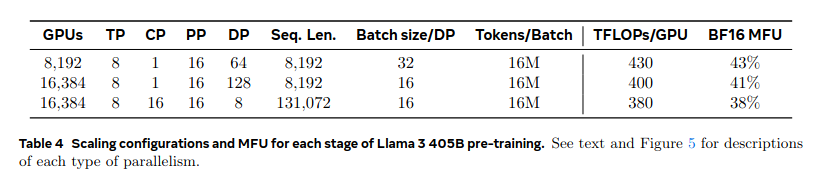
Let’s refer to numbers from the Llama 3 paper, specifically Table 5, which shows three configurations for training Llama-3 405B during pretraining:
Arxiv paper
Looking at the first entry in the table: the global batch size is 16M tokens, the sequence length is 8192, which gives a batch size of 2048 samples. The degree of parallelism (dp) is 64, meaning each micro-batch is of size 32. The paper doesn’t mention gradient accumulation, so I assume it is 1.
Compute
Once you’ve selected the model and defined the total number of training tokens, the compute requirements in terms of floating-point operations (FLOPs) can be estimated. Each compute providers typically advertise their hardware’s peak performance in TFLOPS (trillions of floating-point operations per second).
To estimate the training time, we divide the total number of floating-point operations (FLOPs) required by the peak compute rate (FLOPS) offered by the hardware:
$$ \text{Time (seconds)} = \frac{\text{Total FLOPs}}{\text{Peak FLOPS}} $$With the estimated time and the provider’s cost per second (or per hour), we can then approximate the total training cost.
Some (most?) vendors publish unrealistic peak performance TFLOPS - they aren’t possible to achieve.
However, as Stas Bekman notes in his ML eningeering book, many vendors report optimistic peak TFLOPS values that are rarely achieved in practice. Instead, Model FLOPS Utilization (MFU) should be used to capture how efficiently the hardware is actually being used:
To calculate MFU:
- Measure actual FLOPS achieved: Compute the number of floating-point operations per training iteration, and divide by the iteration time in seconds. This gives actual FLOPS, or effective throughput.
- Compute MFU:
Example
Consider training an LLM on an NVIDIA A100 GPU in FP16 precision. The A100 datasheet, reports a peak of 312 TFLOPS for FP16 precision. If a single iteration of our LLM requires 624 tera‑FLOPs (TFLOPs) and takes 4 seconds, the measured throughput is:
$$ \frac{624\ \text{TFLOPs}}{4\ \text{s}} = 156\ \text{TFLOPS (actual)} $$So the MFU is:
$$ \text{MFU} = \frac{156}{312} = 0.50 \quad (50\% \text{ utilization}) $$In other words, only half the advertised performance is being used. We can then adjust our time and cost estimates by dividing the ideal time by the MFU (or equivalently multiplying the cost by 1/MFU) to reflect realistic estimate of training time and expense.
Acknowledgements
This post draws on insights and examples from the Hugging Face’s book on the Ultra-scale Playbook and Stas Bekman’s book on Machine Learning Engineering. Sincere thanks to both the projects and their contributors for making these resources freely available to the community.