The previous blogs in the series introduced the first and simplest degree of parallelism - data parallelism. Along with optimization from sharding techniques such as ZeRO, LLMs could be trained on a large number of GPUs. But what if LLMs are so large (70B+ parameters) that they cannot fit within the memory of single GPU or even multiple GPUs. This is where pipeline parallelism becomes essential.
The core idea is simple: split the model’s sequential layers across multiple GPUs. For a 24-layer model and 4 GPUs, you might assign:
- GPU 1: Layers 1-6
- GPU 2: Layers 7-12
- GPU 3: Layers 13-18
- GPU 4: Layers 19-24
Each GPU is now a “stage” in the pipeline, responsible for storing and computing only its assigned layers. During the forward pass, activations flow from one stage to the next. During the backward pass, gradients flow in the reverse. However this introduces communication overhead between GPUs to send and recieve activations and gradients. The key challenge in distributed training is to minimize this communication cost or overlap communication with computation.
Naive model parallelism
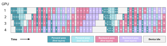
The naive approach to model parallelism would be to distribute the layers across GPU and run the batches of data sequentially. This is how it looks for a single input batch
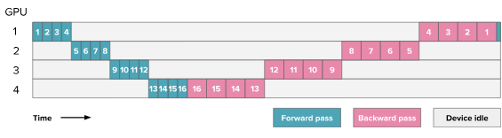
HuggingFace blog. Here the numbers indicate the layers processed for a single batch.
The backward pass (pink boxes) is typically about 2× longer than the forward pass (teal boxes). This is because the backward pass involves two matrix multiplications — one to compute gradients w.r.t. activations, and another for gradients w.r.t. weights whereas the forward pass requires only one.
The way it works is
- Split the model layers across GPUs: For example in the figure above model has 16 layers and there are 4 GPUs: GPU 1 holds layers 1-4, GPU 2 holds layers 5-8, GPU 3 holds layers 9-12 and GPU 4 holds layers 13-16.
- Forward pass: Batch of inputs is sent to GPU 1. GPU 1 computes its layers and produces activations. Once GPU 1 finishes computation, these activations are transferred GPU 2. GPU 2 then performs its layers computations and this continues sequentially across all GPUs. Each stage must wait for the previous stage to finish before starting.
- Backward pass: The gradients computed during backward pass flow in the opposite direction, from the last GPU to the first. Each GPU must wait for the gradient from the next stage before starting its backward computation.
There are several inefficiencies with this naive approach
- Low GPU Utilization (Pipeline Bubbles): At any given time, only one GPU is active while others wait for input from previous stage. The idle time is indicated in gray in the figure above.
- Lack of Computation and Communication Interleaving: GPUs wait for intermediate activations or gradients to be transferred before starting their own computation. Ideally, we’d like to interleave communication (sending data) with computation to hide latency.
- High Memory Demand (Activation Accumulation): Each GPU must cache all intermediate activations for the entire minibatch until the backward pass begins. For large batch size, this quickly becomes a memory bottleneck.
Let \(t_f\) and \(t_b\) be the time to execute forward and backward pass for a single minibatch. The number of micro-batches is \(m\) (for naive case \(m = 1\)), the number of pipeline stages (number of devices used for pipeline parallelism or degree of pipeline parallelism) is denoted as \(p\). The ideal time per iteration is \(t_{id}\). In the case of naive parallelism, the pipeline bubble consists of \(p-1\) forward passes at the start of a batch and \(p-1\) backward passes at the end. The total amount of time spent in the pipeline bubble is
The ideal processing time for all the samples in the batch is the following. Here, the number of micro-batches \(m = 1\).
Therefore, the fraction of ideal computation time spent in the pipeline bubble is
So as we increase the number of GPUs \(p\), idle time grows linearly.Measuring bubble time
GPipe
GPipe paper tackled the bubble problem with a key insight: split the mini-batch into smaller micro-batches.
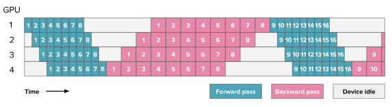
HuggingFace blog. Here the numbers indicate the micro-batches.
The diagram above shows 8 micro batches being proccessed concurrently, keeping every GPU occupied with either forward or backward work. For example, when the first GPU processes a micro-batch, it immediately starts processing second micro-batch. The second GPU starts processing first micro-batch as soon as the first GPU completes processing it.
By keeping the pipeline full of multiple micro-batches, GPipe dramatically improves GPU utilization. However, while GPipe reduces pipeline bubbles, it does not address the other two drawbacks:
- It still does not overlap computation with communication, and
- It retains all activations in memory until the backward phase begins.
Let \(t_f\) and \(t_b\) be the time to execute forward and backward pass for a single minibatch. The number of micro-batches is \(m\), the number of pipeline stages (number of devices used for pipeline parallelism or degree of pipeline parallelism) is denoted as \(p\). The ideal time per iteration is \(t_{id}\). The total amount of time spent in the pipeline bubble is
The ideal processing time for the \(m\) micro-batches is the following
Therefore, the fraction of ideal computation time spent in the pipeline bubble is
Thus, increasing the number of micro-batches \(m\) reduces bubble size proportionally. However, a larger \(m\) also increases memory usage because all microbatch activations must be stored.Measuring bubble time
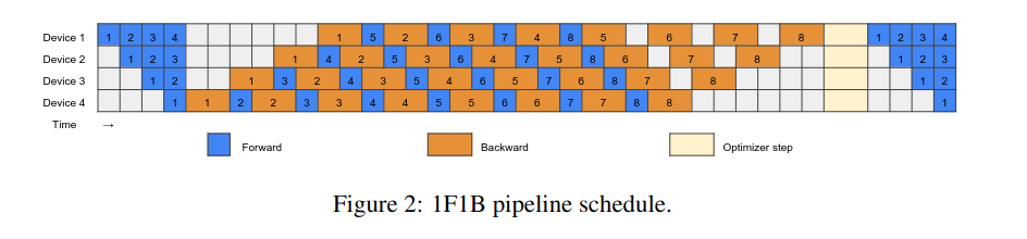
1F1B
One forward one backward (1F1B) schedule helps reduce the activation memory by alternating between forward and backward passes.
As soon as the first micro-batch completes its forward pass through the entire pipeline, the last GPU can immediately start its backward pass. Once the backward computation for a micro-batch is done, its cached activations can be freed, reducing the total memory footprint.
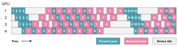
HuggingFace blog
Looking at the figure above, only 4 micro-batches (degree of parallelism) of activation needs to be stored. In contrast, GPipe must store activations for all 8 micro-batches at once. Both approaches process the same number of micro-batches (8), but 1F1B significantly reduces activation memory. This approach does not improve the pipeline bubble observed in the GPipe approach. The bubble still has the same size.
The alternating forward and backward pass means the training loop starts getting complicated as scheduler has to keep track of all the micro-batches and their corresponding forward and backward stages. The 1F1B helps reduce the activation memory but still has the same pipeline bubble time as the GPipe approach.
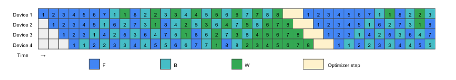
Interleaved 1F1B
To further reduce the bubble size, instead of linear splitting layers across GPUs for the model, the layers of the model are interleaved across devices to form a ring, connecting first and last GPU creating a loop.
If we have a 16-layer model and 4 GPUs, using a modulo scheme based on 4 GPUs:
- GPU 1 → layers (0, 4, 8, 12)
- GPU 2 → layers (1, 5, 9, 13)
- GPU 3 → layers (2, 6, 10, 14)
- GPU 4 → layers (3, 7, 11, 15)
This splits the model into 4 interleaved chunks.
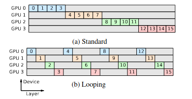
Breadth-First Pipeline Parallelism Figure 3
Looping introduced in Megatron-LM paper improves interleaving and reduces bubble time. Comparing the figures for 1F1B and interleaving 1F1B, the same 8 micro-batches complete faster in interleaving 1F1B compared to only 1F1B. Why is that? How does looping help?
HuggingFace blog A bug in this diagram where backward first layers should be swapped with last layers.
Compared to standard 1F1B, the same 8 micro-batches finish faster because each GPU computes only a small chunk at a time and immediately forwards it to the next GPU. The backward pass works similarly in reverse.
Consider the following: Rough bubble estimates for 1F1B and interleaved 1F1B:
So interleaving reduces the bubble by roughly (old time minus new time)
Interleaving wins if \(\Delta_{bubble} > 0\) i.e.
Plugging some toy numbers in the above equation,
\(K = 4\), \(T_{chunk} = 100 ms\), \(v = 4\) gives RHS = 3 * 100 * (1 − 1/4) = 225 ms.
So if the extra comm/overhead per iteration is \(<\) 225 ms, interleaving should reduce the bubble and improve throughput. If \(C_{comm}\) is larger (e.g., due to very high message latency or many tiny messages), interleaving can lose.Napkin calculation when interleaved 1F1B is faster compared to 1F1B
The training loop is getting more complicated and now model placement requires careful consideration, since layers are no longer sequential. Interleaved 1F1B keeps GPUs busy more consistently, cutting idle time and improving throughput, while still maintaining low activation memory like 1F1B.
The number of micro-batches is \(m\), the number of pipeline stages (number of devices used for pipeline parallelism or degree of pipeline parallelism) is denoted as \(p\). The number of interleaved stages per GPU is \(v\). Each GPU now executes \(v\) smaller stages, so per-stage compute time becomes \(\frac{t_f}{v}\) and \(\frac{t_b}{v}\). The ideal time per iteration is \(t_{id}\). The total amount of time spent in the pipeline bubble is
The ideal processing time for the \(m\) micro-batches is the following
Therefore, the fraction of ideal computation time spent in the pipeline bubble is
Thus, interleaving reduces bubble size by an additional factor of \(v\), at the cost of increased communication.Measuring bubble time
Breadth-First Pipeline Parallelism paper introduces two schedule breadth-first pipeline (BFS) and depth-first pipeline (DFS) – similar to the above interleaved 1F1B. Extracting following excerpt from paper on performance of different schedules
For smaller batches, the breadth-first schedule is by far the most efficient, minimizing both the bubble and network overheads. The depth-first schedule also reduces the pipeline bubble, but its high network overhead makes the performance worse than than the non-looped configurations in most cases. For larger batches, the pipeline bubble is small in all cases, and 1F1B is the fastest because of its lower pipeline-parallel network overhead and memory usage."
Llama 3.1 paper provides insights on how they combine DFS and BFS schedule to optimize the memory and communication efficiently. They also balance the pipeline by reducing transformers layers from first and last stages. First layer is responsible for embedding lookup which increases memory and last layer is used to calculate output and loss which increases the latency.
I don’t understand DFS and BFS schedule clearly. I will revisit those and rewrite for clarity.
Zero Bubble Pipeline Schedule
Zero Bubble paper proposes a clever strategy that eliminates pipeline bubbles by performing fine-grained computation scheduling for the backward pass.
In naive parallelism, we hinted at how backward pass takes roughly about twice as long as the forward pass. This is because the backward pass involves two matrix multiplications — one to compute gradients w.r.t. activations, and another for gradients w.r.t. weights whereas the forward pass requires only one.
The Zero Bubble schedule exploits the fact that weight gradients are not sequentially dependent and can therefore be computed whenever idle compute resources are available. By filling these idle slots with weight-gradient computation, Zero Bubble keeps all GPUs busy and eliminates the pipeline bubbles.
Let’s consider two consecutive linear layers
Here, Let’s denote \(G_{L+1}\) as upstream gradient from the next layer
Backward for layer \(L+1\) consists of two gradients: inputs (B) and weights (W)
Backward for layer \(L\) consists of two gradients: inputs (B) and weights (W)
To compute \(\delta{X_{L}}\) i.e \(B_{L}\), we first need \(dA_{L}\), and to get \(dA_{L}\), we need \(G_{L+1}\). This creates a strict sequential dependency chain \(G_{L+1} -> dA_{L} -> dX_{L} ...\) where Bs depend on the next layer’s B. However, \(dW_{L+1}\) needs only (\(G_{L+1}, A_{L}\)) and \(dW_{L}\) needs only (\(dA_{L}, X_{L}\)). These weights gradients are not required to produce any \(dA\) or \(X\) for earlier layers, so they are off the critical path of the backward chain, and can be scheduled later (any time after their inputs are ready and before optimizer step) to fill the bubbles.Forward and backward computation
Zero bubble paper Figure 2
The figure above shows 1F1B scheduling where there are lot of idle times (white squares). The figure below shows Zero Bubble schedule where nearly all the idle time is eliminated. There’s a complexity here in how these schedules are designed heuristically and synchronizing the gradients for the optimizer step.
Zero bubble paper Figure 3 Zero Bubble Schedule
DeepSeek v3 DualPipe
The DeepSeek v3 paper introduced DualPipe, a technique that overlaps forward and backward computation–communication phases to further reduce pipeline bubbles.
The key idea behind DualPipe is to overlap computation and communication within each pair of forward and backward chunks. Each chunk includes four components — Attention, All-to-All Dispatch, MLP, and All-to-All Combine. The all-to-all operations are introduced by expert parallelism to send and receive data. Similar to the Zero Bubble approach above, the backward chunks for Attention and MLP are split into two parts: backward pass for inputs (B) and backward pass for weights (W).
The figure below illustrates how overlapping computation effectively hides communication latency.
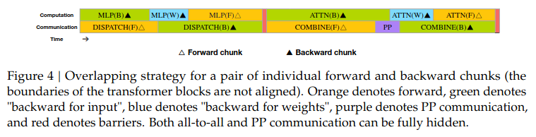
DeepSeek v3 technical paper Figure 4
Figure 5 from the paper illustrates the DualPipe scheduling for 8 pipeline parallelism (PP) ranks and 20 micro-batches, where micro-batches are processed bidirectionally. Until now in all parallelism strategies, micro-batches have been processed in one direction (first microbatch starts at GPU 0, then GPU 1 and so on). In DualPipe, one stream processes forward passes from left to right (GPU 0 -> GPU 1 -> … -> GPU 7). The other, concurrent stream processes forward passes from right to left (GPU 7 -> GPU 6 -> … -> GPU 0).
The schedule is meticulously crafted so that when one microbatch is in its forward pass on a GPU, another microbatch can be in its backward pass on the same GPU. This overlap of forward and backward computations (and their associated communications) is what dramatically reduces the “pipeline bubble” and increases GPU utilization.
This efficiency gain comes at the cost of maintaining two copies of certain model parameters. These duplicate copies are strategically used to facilitate the efficient computation of gradients during the backward pass and enable further overlapping of operations. Why 2x parameters are required?
To run two independent forward passes simultaneously in opposite directions, each device needs to hold two sets of weights for its layer chunks:
- One set for the “forward” pipeline (left-to-right)
- One set for the “reverse” pipeline (right-to-left)
These two sets of parameters are synchronized (their gradients are combined during the backward pass), but they exist as separate copies in memory to allow for the simultaneous, bidirectional computation that defines DualPipe. This memory overhead is the trade-off for the significantly reduced pipeline bubbles and higher training throughput.
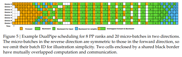
DeepSeek v3 technical paper Figure 5
By running two synchronized pipelines in opposite directions, DualPipe achieves:
- Full overlap of forward and backward communication-computation phases
- Near-zero pipeline bubbles and higher hardware utilization
- Better scaling across many GPUs, especially when combined with expert and tensor parallelism
I would like to explore DeepSeek v3 in depth as part of separate post.
Wrap up
This post introduced a series of pipeline parallelism strategies, each addressing different bottlenecks:
- Naive model parallelism: basic layer-splitting, high idle time.
- GPipe: reduced bubbles via micro-batching.
- 1F1B: reduced activation memory with alternating passes.
- Interleaved 1F1B: finer scheduling, fewer bubbles.
- Zero Bubble: filled idle slots using gradient independence.
- DualPipe: full overlap with bidirectional scheduling.
In practice, pipeline parallelism is almost always combined with data and/or tensor parallelism to achieve truly massive scale. While this post focused on training, pipeline parallelism is also highly effective for inference. Without the need for a backward pass, the scheduling becomes much simpler, allowing for efficient execution of large models across multiple devices.
Pipeline parallelism is particularly valuable for cross-node training, where inter-node bandwidth is often limited. Unlike data parallelism, which requires synchronizing gradients across all nodes, pipeline parallelism primarily passes activations between consecutive stages. This reduces the volume of data sent over the network at any given time, making it easier to utilize bandwidth efficiently and keep GPUs busy even when communication is slower.