Ultra-scale Playbook - Data Parallelism

Hugging Face released a fantastic open-source book for training LLMs on up to 12,000 GPUs.

In the previous post in the ultra-scale series, we looked at what are the different challenges one encounters when training an LLM on a single GPU. There are 4 items that consume memory:

1. Model weights
2. Model gradients
3. Optimizer states
4. Activation required to compute gradients

Activations scale linearly with the batch size and quadratically with the sequence length. We looked into how to optimize the activation memory by using gradient checkpointing and gradient accumulation techniques.

Instead of saving all the activations in the memory during the forward pass, gradient checkpointing reduces the memory footprint by recomputing some of the activations during backward pass. This helps save the activation memory for a single batch size.

Gradient accumulation controls the effective batch size by accumulating gradients over multiple smaller micro-batches before performing a weight update. This technique allows training with larger batch sizes and also highlights a key optimization opportunity – each micro-batch can be processed independently, hence need for using multiple GPUs to parallelize and accelerate training.

The first parallelization strategy that we will be looking at is Data Parallelism.

Data Parallelism

The idea behind data parallelism (DP) strategy is to create replicas of the same model on multiple GPUs and for each GPU, run the forward and backward passes on different micro-batches in parallel.

To ensure consistent model updates across all GPUs, the gradients computed on each GPU must be averaged and synchronized. This is done using a process called gradient synchronization, where gradients are gathered from all GPUs, averaged, and then redistributed so that all model replicas are updated identically.

This synchronization relies on an distributed communication primitive called all-reduce, which performs both the averaging and broadcasting of the gradients across all GPUs in a single step.

HuggingFace playbook contains a parallel computing crash course. It introduces the collective operations such as Broadcast, AllReduce, Scatter and many more required in distrubted computing scenarios.

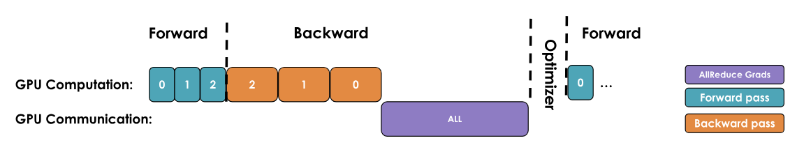
One way to implement the gradient synchronization would be to wait until all micro-batches have completed the forward-and-backward pass, then trigger all-reduce operation across all GPUs, to sync these gradients. This means some of the GPUs will stay idle until the synchronization takes place. This approach wastes the resources.

Notice in the image above, all GPUs remain idle until the communication completes syncing the gradients.

Next, we will take a look three optimization that will reduce the communication overhead and GPU idleness.

Overlap gradient synchronization

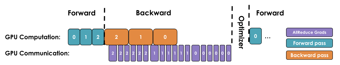
In overlapping gradient synchronization approach, we start syncing the gradients as soon as they are calculated. There is an interleave of communication and computation where we keep calculating the gradients and simultaneously syncing the calculated gradients across all the GPUs.

Here, the gradient synchronization happens in parallel with the backward pass. This approach significantly speeds up the data parallelism training.

Bucketing gradients

The previous idea of syncing gradients as they become available introduces frequent communication overhead. We communicate for every gradient. In bucketing gradients approach, we instead gather gradients in a group and perform all-reduce for all the gradients in the group.

This approach helps reduce the frequency of communication.

Interplay with gradient accumulation

We know how gradient accumulation can simulate the large batch sizes by accumulating the gradients. If we combine gradient accumulation with overlapping and bucketing gradients, we have to be careful on when to sync the gradients. We want to accumulate the gradients from multiple steps during backward pass and then perform the synchronization.

To disable the sync on the backward pass that don’t need reduction, PyTorch provides model.no_sync() decorator.

Implementation

The data parallelism technique is implemented in the Distributed Data Parallelism module for PyTorch.

PyTorch DDP module takes care of bucketing and synchronizing the gradients. The internal design documentation provides further insights on the exact mechanics take during construction, forward pass, backward pass and optimizer step.

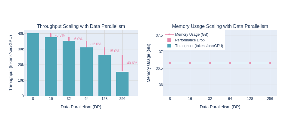
Limitations

As we scale the DDP setup to larger GPUs, the benefits offered by DDP being to break down. The overhead of communication between all the devices becomes significant as we add more GPUs. This limit is reached mainly because of how data parallelism approach works

1. Every GPU holds a full copy of the model: Each GPU device has its own replica of model states - all model parameters, it’s own optimizer states, and during the forward/backward pass it computes gradients for exactly the same set of parameters.

2. Gradients must be syncronised every iteration: After calculating the gradients for each microbatch, the “local” gradients must be synced across all GPU devices. This is usually done using “all-reduce” distributed operation. Once all gradients are synced, we update the model parameters.

DDP works well if we have model that fits a single GPU and a batch of data having at least 1 sample. However, DDP reaches its limits when either the model becomes too large to fit into a single GPU, or when the data (e.g., long sequences) exceeds the memory capacity of the device.

There are two orthogonal approaches that can be applied independently or combined together to scale model training: sharding and parallelism.

• Sharding: Typically sharding involves reducing the memory consumption of each GPU by partitioning the training components such as model weights, gradients, and optimizer states across all GPU devices. Popular implementations include PyTorch FSDP, FSDP2 or DeepSpeed ZeRO.

• Parallelism: This refers to dividing the computation graph or model structure itself across GPUs, so that different parts of the model are executed on different devices. The most common types include tensor parallelism, pipeline parallelism, context parallelism and expert parallelism.

In the next blog, we will look into sharding.