In the previous post of this series, we looked at how data parallelism lets us distribute LLM training across many GPUs. Data parallelism (DP) is memory-inefficient because model states - model parameters, gradients and optimizer states are redundantly stored on every GPU. This memory consumption can be significantly reduced using sharding techniques such as Zero Redundancy Optimizer (ZeRO). The various ZeRO strategies help reduce the memory consumption by partitioning the model states - the model parameters, gradients and optimizer states across GPUs.
Before looking into the optimization techniques, let us remind ourselves what are the sequence of operations performed to take a single training step using data parallelism technique:
- Forward pass: Each GPU runs a forward pass on its full model replica with its micro‑batch.
- Backward pass: Each GPU computes local gradients for all parameters.
- Gradient synchronization: An all‑reduce, usually ring all-reduce, is performed using reduce‑scatter + all‑gather operation to average gradients across GPUs.
- Optimizer step: Each GPU applies its full optimizer state to the averaged gradient and updates its local weights.
- Model parameter update: Updated parameters are already global and no additional communication is needed.
We will look into 3 optimization stages of ZeRO techniques and how they partition the model states.
ZeRO
Stage 1
Instead of each GPU holding an entire copy of optimizer state, in ZeRO-1, the optimizer state is partitioned across data parallel processes. The gradient and model parameters are fully replicated and only the optimizer states are sharded. The sequence of operations for single training step using ZeRO stage 1 optimization is the following:
- Forward pass: Full forward on each replica as in DP.
- Backward pass: Similar to the data parallelism second step, the local gradients computed per GPU.
- Gradient synchronization: It performs reduce-scatter operation on the gradients. Reduce-scatter is a collective operation that combines reduction (summing/averaging gradients) and scattering (sharding results).
- Optimizer step (sharded): Each GPU updates only its shard of the optimizer state and corresponding parameter slice using its gradient shard.
- Model parameter synchronization (parameter all-gather): Each GPU holds only a slice of updated parameters, so it performs an all-gather to reconstruct the full BF16 model locally
ZeRO-1 offers reduced optimizer-state memory by a factor of N (where N = number of data-parallel GPUs). Both ZeRO-1 and vanilla DP use the same communication volume (a combination of reduce-scatter and all-gather applied in different places).
Stage 2
In Stage 2, sharding goes one step further: alongside optimizer states, gradients are also partitioned. For each micro-batch, a particular GPU maintains gradients only for a subset of model parameters. Each GPU therefore holds only a subset of gradients, cutting memory use compared to Stage 1’s full replication.
To update the model parameters, each GPU no longer requires the full gradient tensor but only the relevant shard of gradients corresponding to the parameter slices it owns. The sequence of operations for a single training step using ZeRO-2 optimization is as follows:
- Forward pass: Same as DP and ZeRO-1, each GPU runs a full forward pass with the entire model.
- Backward pass: Each GPU computes local gradients, but instead of keeping all gradients, it prepares for gradient sharding.
- Gradient synchronization (sharded): A reduce-scatter operation is performed on the gradients, which simultaneously aggregates and partitions the gradients across GPUs. After this step, each GPU only holds a shard of the full gradient.
- Optimizer step (sharded): Each GPU updates only its own shard of the optimizer state and the corresponding parameter slices using its local gradient shard.
- Model parameter synchronization (parameter all-gather): Since each GPU holds only a slice of the updated parameters, an all-gather operation reconstructs the full model parameters locally on each GPU for the next forward pass.
Here’s how it looks like
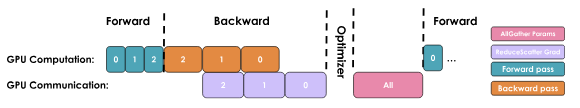
HuggingFace blog
There is no communication overhead in ZeRO-2 compared to ZeRO-1 and vanilla data parallelism, as all approaches use the same reduce-scatter and all-reduce operations just applied differently.
The distributed communication blog introduces these operations in detail.
Stage 3
Both ZeRO-1 and ZeRO-2 provide substantial memory savings by sharding optimizer states and gradients, but they assume that the full model parameters can still fit on each GPU. This assumption breaks down for ultra-large models of size hundreds of billions of parameters where even a single forward or backward pass exceeds the GPU memory capacity.
ZeRO-3 solves this by sharding model parameters as well, so no GPU ever stores the full model. With this, all three components of model state optimizer states, gradients, and parameters are sharded across the data-parallel devices. No GPU holds a full replica of the model at any time, making it possible to train truly massive models that would otherwise be impossible to fit. The sequence of operations in ZeRO Stage 3 is as follows:
- Forward pass (with parameter gathering): Since parameters are sharded, each GPU first gathers the relevant parameter shards needed for its portion of the forward pass.
- Backward pass: Similar to the forward pass, parameter shards are gathered as needed to compute local gradients.
- Gradient synchronization (sharded): Gradients are aggregated and sharded across GPUs, just like in ZeRO-2.
- Optimizer step (sharded): Each GPU updates only its shard of the optimizer state and model parameters using the local gradient shard.
The gradient and optimizer step work similar to ZeRO-2. Two extra all-gather operations are added during forward and backward pass to gather the layer parameters. Consider the following example: with four layers distributed across four GPUs, ZeRO-3 shards parameters as shown below:
| GPU | Parameter Shard |
|---|---|
| GPU 0 | Layer 0 |
| GPU 1 | Layer 1 |
| GPU 2 | Layer 2 |
| GPU 3 | Layer 3 |
Each GPU is assigned a layer’s parameters and owns the optimizer states and gradients only for that layer. During forward pass where each replica is processing micro-batches, to compute Layer 0, all GPUs gather Layer 0 parameters from GPU 0, compute the forward output for Layer 0 using their micro-batch, and store the activations for use in the backward pass. Once Layer 0 is complete, the gathered parameters are discarded to save memory. This process repeats layer by layer. During the forward pass, no GPU ever holds the entire model in memory. It only gathers one layer’s parameters at a time, computes forward, and moves on.
During the backward pass, the process is reversed. Starting from Layer 3, each GPU gathers Layer 3 parameters from GPU 3, recomputes any intermediate results if needed (unless stored), and computes the gradient using the stored activation. This gradient is then reduce-scattered to the owning GPU (in this case, GPU 3), which keeps only the shard relevant to its layer. This process continues backward through all layers. Each GPU accumulates gradients only for the layer it owns.
Once backward pass is complete, each GPU updates only its shard of the optimizer state and its own layer’s parameters, using the gradients it owns. Since gradients and optimizer states are sharded, this update step is done entirely locally and no communication is required.

ZeRO stage-3 example
Stas Bekman’s guide on ZeRO-DP strategies provides an alternate example demonstrating ZeRO-3 optimization. It splits the layers at tensor level where a single layer’s weights might be split across multiple GPUs.
Here’s how it looks like
HuggingFace blog
With additional communication overhead, ZeRO-3 offers significant memory reduction by partitioning all model states.
Implementation
Both Deepspeed library and PyTorch library support various ZeRO stage implementations.
PyTorch refers to ZeRO-3 stage as FullyShardedDataParallel FSDP. It takes a different implementation approach compared to ZeRO-3 implementation in DeepSpeed. PyTorch provides two FSDP implementations: FSDP1 and FSDP2. There are advanced optimization strategies such as ZeRO Infinity and ZeRO++ as part of Deepspeed library.
The implementation frameworks hide the effective communication overhead optimally by overlapping the computations and communications.
Summary
So far, we’ve explored three ZeRO stages for data-parallel training, each trading off a bit of extra communication for huge memory savings.
Arxiv paper
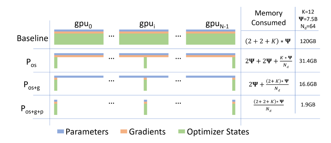
The figure from the paper compares per-device memory consumption using the 3 ZeRO-DP optimization stages. For a 7.5 billion parameter model and a 64 degree data parallelism (number of GPUs used), vanilla data parallelism strategy requires 120 GB memory. Comparing the various ZeRO strategies, \(P_{os}\) refers to optimizer state partitioning, ZeRO-1 stage requires 31.4 GB of memory ~ 4x reduction. ZeRO-2 stage, \(P_{os+g}\) refers to optimizer state and gradient partitioning reduces the memory footprint further down to only 16.6GB of memory ~ 8x reduction. Lastly, ZeRO-3 stage, \(P_{os+g+p}\) refers to parameter, optimizer state and gradient partitioning takes only 1.9 GB of model-state memory ~ 64x reduction.
Key Takeaways
- The model parameters and gradients are replicated in stages ZeRO-1 and optimizer sharded.
- Likewise for ZeRO-2 stage, model parameters are replicated but gradients and optimizer states are shared.
- All model states are sharded in ZeRO-3 stage.
Using the ZeRO and DP techniques, we can train larger models on multiple GPUs where models cannot even fit on a single GPU. We can scale the training using the combination of ZeRO and DP approach by adding more replicas. This works only assuming we can fit a single layer on a single GPU. Recall in the first part of the series, we looked at how activation memory becomes a memory bottleneck for larger sequence size and batch size. This is where other axis of parallelism helps where we also partition activation memory.
We will look into different parallelism approaches such as model, tensor, context, sequence and expert parallelism on next in the series.