The post on post-training SFT covered four finetuning experiments on direct and reasoning tasks using LoRA and full-finetuning approaches. This post covers different reinforcement learning (RL) approaches used in post-training.
SFT teaches a model by giving it examples to imitate. The training data contains target responses, and the model learns to generate tokens from the target distribution.
RL takes a different approach. Instead of showing the model exactly how to solve a problem, we let it generate solutions, evaluate how good those solutions are, and update the model so that successful behaviour becomes more likely.

Reinforcement Learning (RL)
I would recommend reading the RLHF book by Nathan Lambert.
Standard RL
A standard RL setup consists of environment, agent, action, policy, state and reward.
- Agent: the system making decisions.
- Environment: the world the agent interacts with.
- State: the current condition of the environment.
- Action: a decision made by the agent.
- Policy: the function used by the agent to choose an action.
- Reward: feedback describing how useful an action or trajectory was.
- Trajectory: a sequence of states and actions produced while interacting with the environment.
At each timestep, the agent observes the current state, samples an action from its policy, and performs that action in the environment. The environment transitions to a new state and returns a reward. The objective is to learn a policy that maximises the expected cumulative reward.
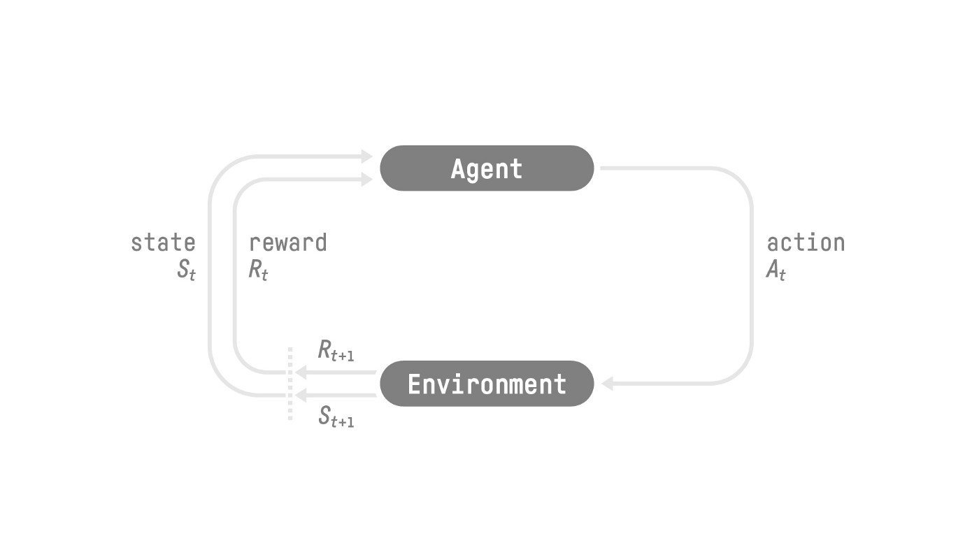
Reinforcement Learning: An Introduction, Richard Sutton and Andrew G. Barto
A policy can be stochastic like a deep learning network learned function or deterministic returning same action for a given state.
A classic example for deterministic policy would be navigating a grid. A fixed policy would be like if state == bottom_left_of_grid, always move right. For a given state, the policy always chooses the same action.
Alternatively, an example of stochastic policy would be playing Atari breakout game. A stochastic policy represents distribution over actions P(right) = 0.7, P(up) = 0.2 and P(left) = 0.1. The agent samples an action from this distribution.
Language models naturally fit the stochastic formulation because, given some text, the model produces a probability distribution over the next token.
RL for Language Models
In many LLM post-training setups, there is no external environment in the classical sense. There are two useful ways to map the RL formulation onto language generation.
Response level : At response level, the model receives a prompt sampled from the training dataset, generates a completion and receives a reward upon completion. RL components are
- input prompt as the context
- entire completion as the action
- LLM as the policy
- reward as scalar score for the completion
A (prompt, completion) pair is commonly referred to as a rollout or trajectory.
Token level : At token level, generation can instead be viewed as a sequence of state transitions. For example,
state_0 = prompt
action_0 = token_1
state_1 = prompt + token_1
action_1 = token_2
- state becomes input prompt + tokens generated so far
- action will be next generated token
- policy will be probability distribution over the next token
The complete generated sequence forms the trajectory. The interesting difference from supervised learning is that RL does not tell the model which token it should have generated. Instead, the model generates its own trajectory and receives feedback describing how good that trajectory was.
RLHF
Reinforcement Learning from Human Feedback (RLHF) adapts the standard RL setup for finetuning LLM when desired behaviour cannot be expressed as programmatic reward function. There are no simple reward functions that could answer questions like which answer is more helpful? which answer is more creative? or which writing style human would prefer?
RLHF training is a two-step process:
- Reward Model (RM): Train a reward model using human preference data. The model generates multiple candidate responses. And the responses are ranked (or compared) by human annotators. These comparisons are used to train a RM. The reward model learns to predict a scalar value (reward) for a given text on how likely would human prefer the output. A higher value should correspond to a response humans are more likely to prefer.
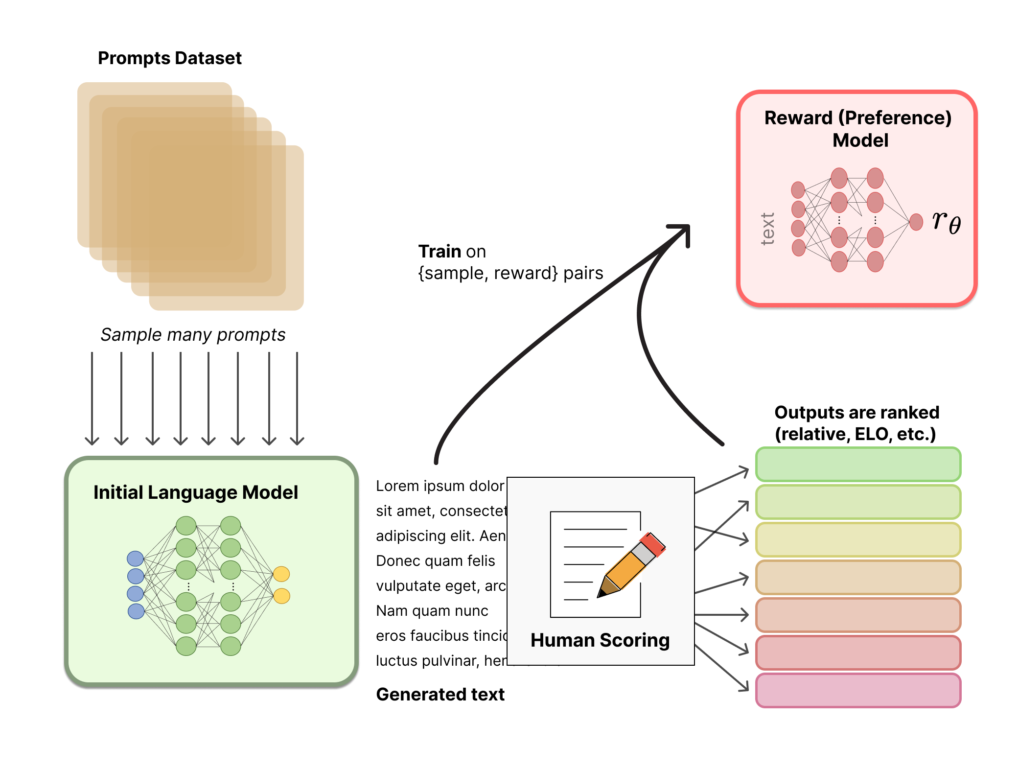
Illustrating Reinforcement Learning from Human Feedback (RLHF)
- Optimising with RL: In this second step, RL is used to optimise the LLM using reward model. The setup consists of initial LLM frozen from SFT stage as reference model. Trainable copy of same model is referred as the policy model. The policy generates responses, the reward model scores them, and policy weights are updated to make high-reward response more likely.
A Kullback–Leibler (KL) divergence term is applied to penalize policy model if it moves away from reference model. Without such a constraint, the policy may exploit weaknesses in the learned reward model rather than genuinely producing better responses.
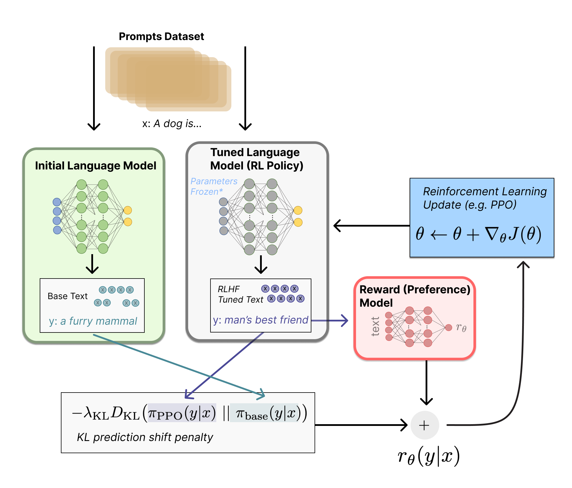
Illustrating Reinforcement Learning from Human Feedback (RLHF)
Policy Gradient Algorithms
The reward tells us whether an output was good or bad, but we still need an algorithm that converts that reward signal into updates to the model weights.
This is where policy gradient algorithms such as PPO, GRPO and many other policy optimisation (PO) algorithms come in.
The general idea behind policy gradient to update LLM weights is
- Generate output using the current policy
- Calculate reward
- Estimate an advantage
- Increase probability of good actions or decrease probability of bad actions
The advantage measures how much better or worse a sampled action or trajectory performed compared with some baseline. Different RL algorithms differ in how this baseline is estimated and how aggressively the policy is allowed to change.
PPO model uses critic/value model to estimate the expected future reward. This estimate is then used as a baseline when calculating the advantage. Traditional PPO-based RLHF involves four conceptual model roles: a trainable policy, a trainable value/critic model, a frozen reward model, and a frozen reference policy. The reward model is trained beforehand and the RL stage updates the policy and critic.
Group Relative Policy Optimisation (GRPO), introduced in the DeepSeekMath work, simplifies by removing the need to train a critic model. Instead of training a value model, GRPO generates a group of responses for the same prompt. Each completion can then be evaluated relative to other completions in the same group.
$$ A_i = \frac{r_i - \mu_r}{\sigma_r}, \qquad \mu_r = \frac{1}{G}\sum_{j=1}^{G} r_j $$A completion that performs better than the group average receives a positive advantage, while one that performs worse receives a negative advantage. The policy is then updated to make higher-advantage trajectories more likely.
One important consequence is that groups where every completion receives the same reward provide no relative learning signal.
For a more detailed comparison of policy-gradient algorithms and their advantage estimators, I recommend the policy gradient chapter of Nathan Lambert’s book.
Reinforcement Learning with verifiable rewards (RLVR)
RLHF is useful when evaluating an answer is subjective. RLVR provides another way to scale RL using verifiable rewards for certain reasoning tasks. The verifiable rewards are functions. For code these functions are unit tests. For maths, these functions are the final expected answer.
Instead of learning a reward model from human preferences, RLVR uses a deterministic verifier. The model generates a solution, the verifier executes it, and the result becomes the reward. The model is now generating the data used to improve itself. This makes code and mathematics particularly attractive domains for RL because we can generate and evaluate large numbers of rollouts without requiring humans to label every response. GRPO, PPO or another policy-gradient algorithm can be used with verifiable rewards.
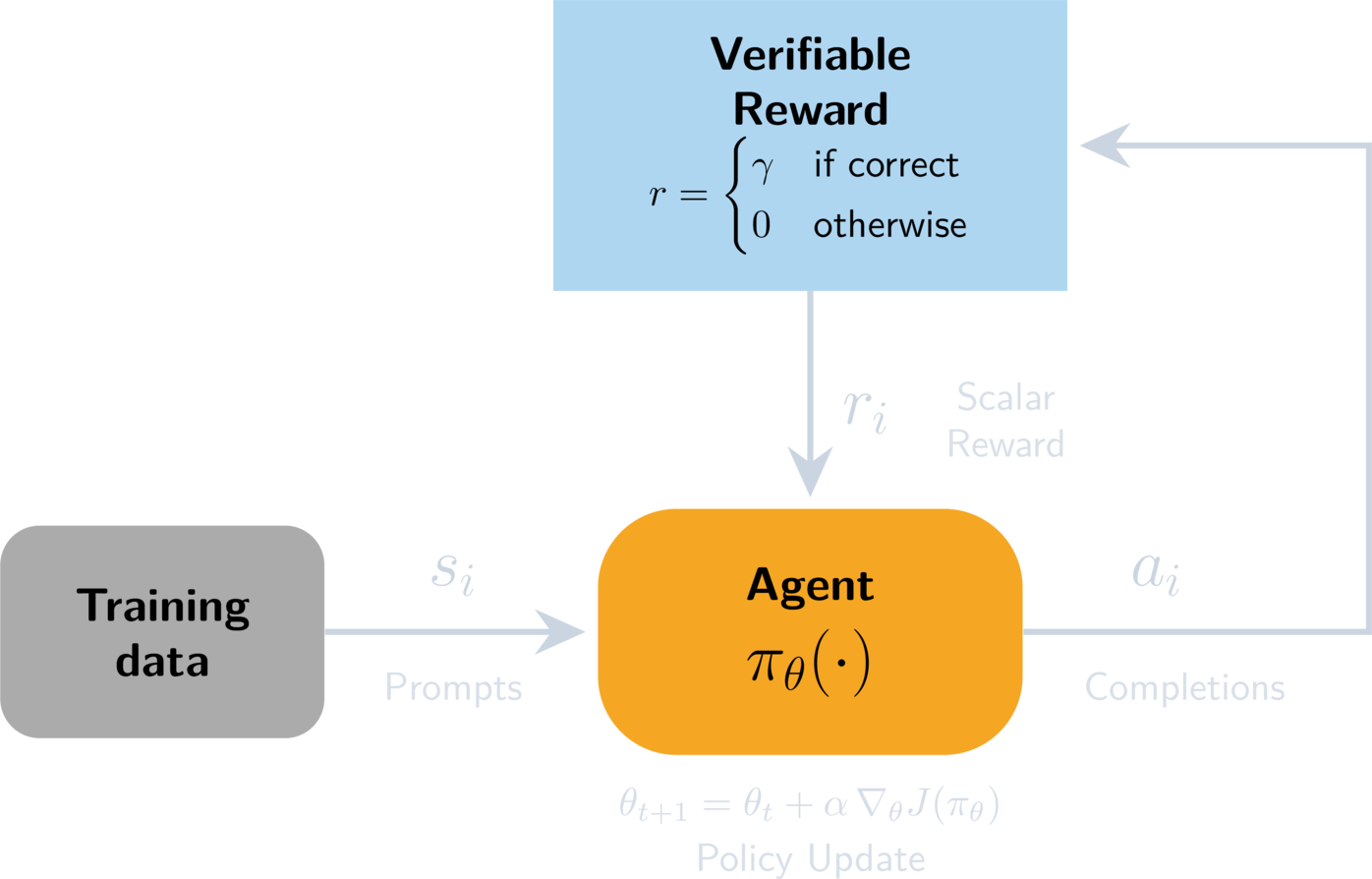
This is where RL environments play a significant role in scaling the RLVR training. RL environments provide the external state, tools, observations and execution context needed to evaluate or continue a trajectory. For code RLVR, the policy may generate code on a rollout server while a sandbox environment executes that code against tests and returns the resulting reward.
Here’s link to a guide comparing various RL environment libraries.
Example
A simple way to understand the difference between SFT, RL and on-policy distillation is to ask two questions:
- Who generates the trajectory the student trains on?
- Where does the learning signal come from?
Consider a model learning to answer: Solve: 17 × 13
SFT: learn from the teacher’s solution
In supervised fine-tuning, the training dataset already contains the response that the model should produce. The target may have been written by a human or generated by a stronger model. For example, the dataset could contain either
a direct answer: Answer: 221 or a reasoning trace:
17 × 10 = 170
17 × 3 = 51
170 + 51 = 221
Answer: 221
The student is trained with next-token prediction on this fixed response. The teacher generates a trajectory and the student imitates trajectory. Every target token provides supervision. If the teacher writes 51, the training objective increases the student’s probability of producing 51 given the preceding tokens. This makes SFT information-dense and efficient. However, the student trains on states visited by the teacher.
Suppose that at inference time the student instead produces:
17 × 10 = 170
17 × 3 = 41  -> mistake here
The model is now conditioning on a prefix that may never have appeared in the SFT dataset. The teacher would not normally generate the mistake 41, so the student receives little training on how to recover from states created by its own errors. In the terminology used here, SFT is off-policy with respect to the student: the training states come from human or teacher trajectories rather than trajectories sampled from the current student policy.
RL: learn from the student’s own attempts
Reinforcement learning reverses who generates the training trajectory. The student attempts the problem itself.
Student generates:
17 × 10 = 170
17 × 3 = 41
170 + 41 = 211
Answer: 211
The trajectory is then evaluated: reward = 0. Another rollout might produce: reward = 1 for
17 × 10 = 170
17 × 3 = 51
170 + 51 = 221
Answer: 221
The successful trajectory receives a higher advantage, and the policy-gradient algorithm updates the model so that actions associated with successful trajectories become more likely. The student generates a trajectory, the environment evaluates it and student learns from the reward. This is on-policy because the model learns from trajectories produced by its own policy.
The advantage is that training follows the model into the states it actually visits. As the model improves, it generates new and potentially better training data. The downside is that the reward may contain much less information than an SFT target. If a 2,000-token reasoning trace receives reward = 0, we know that something went wrong, but the reward does not necessarily tell us which token or reasoning step caused the failure. The policy-gradient algorithm still produces token-level gradients, but credit assignment from a trajectory-level reward can be difficult.
RLVR: RL with an objective verifier
RLVR is a special case of RL where the reward comes from something that can be checked automatically. For this multiplication example, the verifier could simply compare the final answer with the expected answer:
if generated_answer == 221:
  reward = 1
else:
  reward = 0
For code, the verifier could instead execute the generated program against unit tests:
if all_unit_tests_passed == True:
  reward = 1
else:
  reward = 0
The important difference from SFT is that there is no need for a teacher to demonstrate how the problem should be solved. The student is not required to imitate a particular demonstrated solution and can potentially discover alternative successful strategies. The verifier only cares whether the result satisfies the task.
This gives RLVR an interesting property: the student can potentially discover successful behaviours that were never present in a teacher’s demonstrations. Its weakness is still the sparsity of the learning signal. A final pass/fail result tells the model whether a trajectory worked, but often not where it went wrong.
On-policy distillation: let the student drive, but let the teacher correct it
On-policy distillation combines aspects of SFT and RL. Like RL, the student generates its own trajectory. Suppose the student produces:
17 × 10 = 170
17 × 3 = 41
Instead of only receiving: reward = 0 a stronger teacher model evaluates the student’s actual prefix.
At:
17 × 3 =
the distributions might look like:
Student:
P(41) = 0.65
P(51) = 0.10

Teacher:
P(41) = 0.001
P(51) = 0.97
The teacher therefore provides a strong learning signal precisely at the state where the student’s behaviour diverged. The student first generates its own trajectory. The teacher produces its token distribution at each student-visited state, and the distillation objective pushes the student’s distribution toward the teacher’s.
This is also on-policy, because the states being trained on came from the student. But unlike RLVR, the feedback is dense. Instead of receiving one scalar reward for the whole trajectory, the student can receive information at every generated token.
Analogy
A useful analogy is:
SFT: Watch an expert solve the problem and imitate them.
RLVR: Solve the problem yourself and only check whether the final answer is correct.
On-policy distillation: Solve the problem yourself while an expert watches each step and tells you how they would act from the exact state you reached.
Inspired by Will Brown’s post on comparing SFT, RL and OPD.
Experiment
For this experiment, I start from the corresponding full-finetuned SFT checkpoints from the previous experiment and ask a narrower question:
Can RLVR improve code correctness beyond SFT?
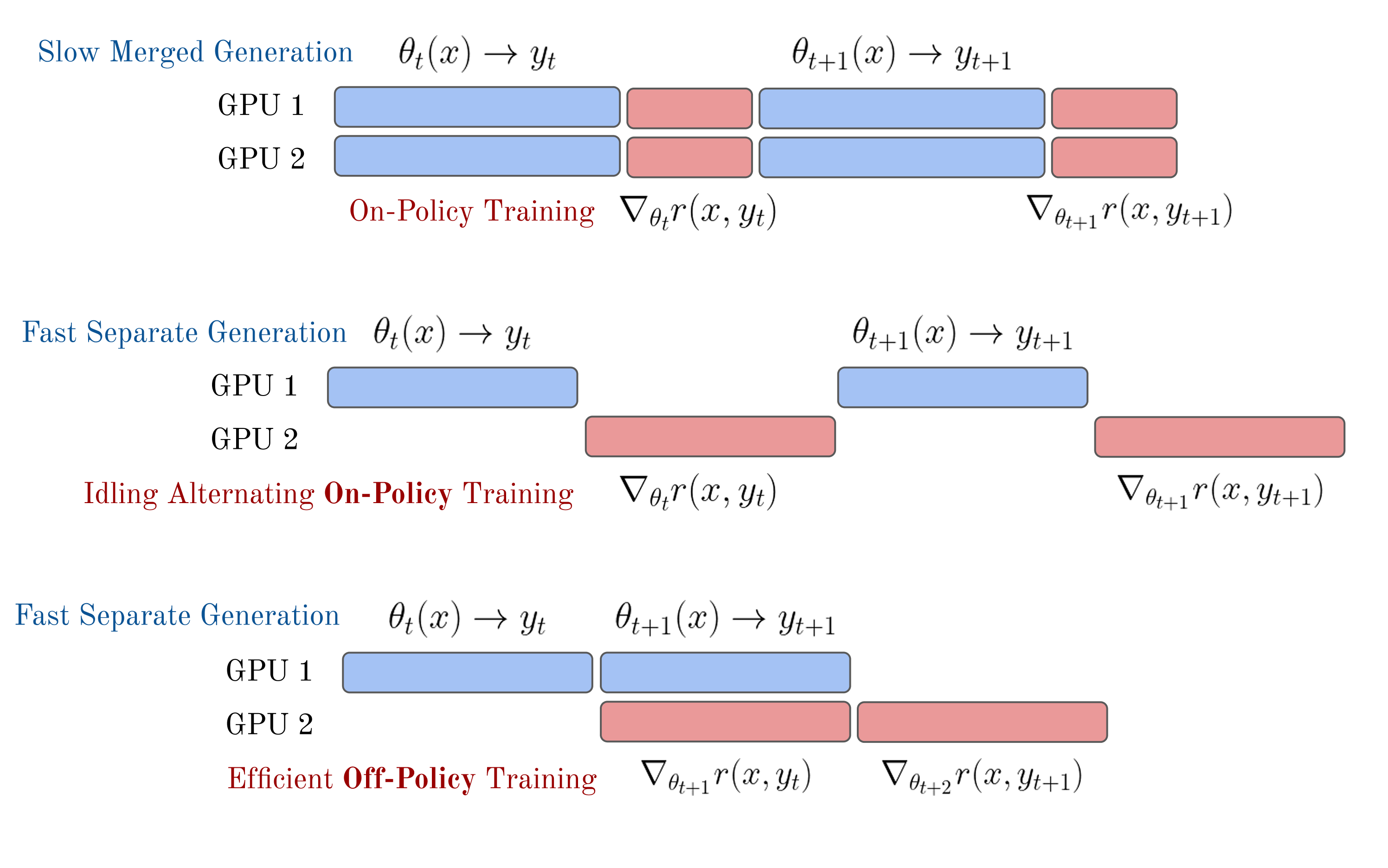
RL training infrastructure consists of two approaches
- Sync RL training
Training waits for the current batch of rollouts to finish before updating the policy. This keeps the generated data relatively fresh because the model used to produce the rollout is close to the model being updated. The downside is utilisation. Generation can be slow, particularly for long reasoning traces, and training hardware may spend time waiting for rollout generation to finish.
- Async RL training
Asynchronous RL overlaps rollout generation and optimisation. This can improve hardware utilisation but introduces policy staleness: some rollouts may have been generated by an older version of the model than the one currently being trained.
Training Setup
The RL dataset is based on KodCode-Light-RL-10K. The dataset is filtered using similar decontamination approach against benchmark dataset described in SFT project.
The code for RLVR: https://github.com/dudeperf3ct/minicode-llm/tree/main/rlvr
Weights & Biases experiments: https://wandb.ai/dudeperf3ct/qwen35-4b-kodcode-rlvr
Hugging Face models: https://huggingface.co/dudeperf3ct/qwen35-4b-kodcode-rlvr-1k
I use Axolotl to train the RLVR models. For each prompt, the policy generates eight completions. Generated Python is then executed against the problem’s public tests inside isolated Modal Sandboxes. The code reward is binary
reward = 1 if all_tests_pass else 0
The two experiments start from the matching full-finetuned SFT checkpoints. The names direct-fft and reasoning-fft refer to those starting checkpoints; the RL update itself uses LoRA with rank 32. Both runs use the same 1,000 training prompts, seed 42, one epoch and eight rollouts per prompt. One H100 serves rollouts with vLLM, while a second H100 performs training. Generated code is evaluated in isolated Modal Sandboxes.
The direct run uses GRPO with a binary code reward, non-thinking generation and maximum completion length of 2048.
The reasoning run uses Dr. GRPO with thinking generation, 8192 maximum length and the same code reward with an additional 0.05-weighted format reward for producing a closed reasoning trace followed by valid Python. The format reward encourages the reasoning model to produce a closed reasoning trace followed by syntactically valid Python.
Training Results
The current evaluation artifacts use the first scheduled checkpoint from each run: step 500 for direct generation and step 250 for reasoning. Mean code reward is the fraction of sampled completions that passed all public tests for their training problem.
| Run | RL update | Evaluated checkpoint | Mean code reward | Mean format reward | Mean completion tokens | Time to checkpoint |
|---|---|---|---|---|---|---|
| Direct SFT (FT) → RLVR | GRPO + LoRA | 500 | 0.3685 | — | 802 | 20h 12m 53s |
| Reasoning SFT (FT) → RLVR | Dr. GRPO + LoRA | 250 | 0.4445 | 0.8530 | 3,256 | 20h 29m 6s |
The reasoning run produces much longer completions: around 3,256 tokens on average compared with 802 for direct generation. This also illustrates why rollout generation quickly becomes one of the expensive parts of reasoning RL.
Eval Results
All results are percentages. HumanEval, HumanEval+, MBPP and MBPP+ report pass@1, while LiveCodeBench reports accuracy.
SFT Baselines
These values are copied from the previous SFT experiment for comparison.
| Experiments | HumanEval | HumanEval+ | MBPP | MBPP+ | LiveCodeBench Easy | LiveCodeBench Medium | LiveCodeBench Hard |
|---|---|---|---|---|---|---|---|
| Base → direct SFT (LoRA) | 75.00% | 70.12% | 63.76% | 54.76% | 64.87% | 15.11% | 3.33% |
| Base → direct SFT (FT) | 82.32% | 77.44% | 65.34% | 56.88% | 63.44% | 19.03% | 1.85% |
| Base → reasoning SFT (LoRA) | 85.98% | 76.83% | 82.54% | 70.90% | 80.65% | 34.44% | 6.30% |
| Base → reasoning SFT (FT) | 84.76% | 78.66% | 80.42% | 67.20% | 78.49% | 36.86% | 7.04% |
RLVR Checkpoints
The direct checkpoint uses greedy non-thinking decoding.
The reasoning checkpoint uses thinking mode with temperature 0.6 and one sample per problem, matching the corresponding SFT evaluation profiles.
| Experiments | HumanEval | HumanEval+ | MBPP | MBPP+ | LiveCodeBench Easy | LiveCodeBench Medium | LiveCodeBench Hard |
|---|---|---|---|---|---|---|---|
| Direct SFT (FT) → RLVR (LoRA, step 500) | 79.27% | 74.39% | 66.40% | 56.08% | 63.80% | 18.13% | 1.85% |
| Reasoning SFT (FT) → RLVR (LoRA, step 250) | 81.71% | 75.61% | 80.42% | 69.05% | 81.00% | 34.74% | 7.78% |
The percentage-point changes below compare each RLVR checkpoint only with its matching full-finetuned SFT starting checkpoint.
| RLVR checkpoint vs. matching SFT checkpoint | HumanEval | HumanEval+ | MBPP | MBPP+ | LiveCodeBench Easy | LiveCodeBench Medium | LiveCodeBench Hard |
|---|---|---|---|---|---|---|---|
| Direct, step 500 | -3.05 | -3.05 | +1.06 | -0.80 | +0.36 | -0.90 | 0.00 |
| Reasoning, step 250 | -3.05 | -3.05 | 0.00 | +1.85 | +2.51 | -2.12 | +0.74 |
Learnings
- Reported and patched few bugs in axolotl library
0.18.0. - The Async GRPO approach in axolotl library was broken so I had to stick with synchronous RL training approach. I had to manually maintain patches as part of this experiment.
- Neither checkpoint shows a broad correctness improvement over its SFT starting point.
- The direct checkpoint improves MBPP and LiveCodeBench Easy slightly, but regresses on HumanEval, HumanEval+, MBPP+ and LiveCodeBench Medium.
- The reasoning checkpoint improves MBPP+, LiveCodeBench Easy and LiveCodeBench Hard, holds MBPP flat, and regresses on both HumanEval variants and LiveCodeBench Medium.
- These results come from one seed and intermediate checkpoints.
There could be several possible explanations:
- RL dataset is small: Each run only uses 1_000 unique prompts. With 8 rollouts per prompt, the model can generate 8_000 trajectories.
- Binary rewards are sparse
- Not every rollout group produces a gradient signal: GRPO relies on differences between rewards within the same group. For example, of all eight rollouts fail: [0, 0, 0, 0, 0, 0, 0, 0] there is no relative advantage. The same is true if all eight succeed. As the policy becomes either too weak or too strong for a problem, that prompt stops providing useful relative-learning signal.