Transfer Learning

In this post, we will go through basics of Transfer Learning using Cats vs Dogs Redux Competition dataset from kaggle. We will implement this using one of the popular deep learning framework Keras .

All the codes implemented in Jupyter notebook in Keras, PyTorch, and fastai.

All codes can be run on Google Colab (link provided in notebook).

Hey yo, but what is Transfer Learning?

Well sit tight and buckle up. I will go through everything in-detail.

Feel free to jump anywhere,

Learning Curves
Introduction to Transfer Learning
- Transfer Learning scenarios
- When and how to finetune?
Recap
Keras
- ConvNet as feature extractor
- Finetuning
Further Reading
Footnotes and Credits

Dogs vs Cats Redux dataset

The train folder contains 25,000 images of dogs and cats. Each image in this folder has the label as part of the filename. The test folder contains 12,500 images, named according to a numeric id. For each image in the test set, the task is to predict a probability that the image is a dog (1 = dog, 0 = cat).

Data Preprocessing

Getting a data from kaggle using Kaggle API is a little tricky part. For brevity, I will leave that part in notebooks and suppose that all data is downloaded.

The dataset once unzipped we get the data in following directory structure.

data/
   train/
     dog001.jpg
     dog002.jpg
     …
     cat001.jpg
     cat002.jpg
     …
   test/
     001.jpg
     002.jpg
     …

We will convert the above directory structure into this structure for ease of data processing. Also, split the training data into train and validation sets.

data/
   train/
     dogs/
       dog001.jpg
       dog002.jpg
       …
     cats/
       cat001.jpg
       cat002.jpg
       …
   val/
     dogs/
       dog121.jpg
       dog112.jpg
       …
     cats/
       cat111.jpg
       cat102.jpg
       …
   test/
     001.jpg
     002.jpg
     003.jpg
     …

print ('Training set images', len(os.listdir(train_cats_dir))+len(os.listdir(train_dogs_dir)))
print ('Validation set images', len(os.listdir(val_cats_dir))+len(os.listdir(val_dogs_dir)))
print ('Test set images', len(os.listdir(test_path)))

Training set images 20000
Validation set images 5000
Test set images 12500

Visualization of data

Enough talk, show me the cats and dogs!

def preprocess_img(img, ax, label, train_dir):
    im = Image.open(os.path.join(train_dir, img))
    size = im.size
    ax.imshow(im)
    ax.set_title(f'{label} {size}')

train_x = os.listdir(train_cats_dir)
# plot the images in the batch, along with the corresponding labels
fig = plt.figure(figsize=(25, 10))

for idx in np.arange(10):
    ax = fig.add_subplot(2, 10/2, idx+1, xticks=[], yticks=[])
    preprocess_img(train_x[idx], ax, 'cat', train_cats_dir)
    # print out the correct label for each image

train_x = os.listdir(train_dogs_dir)
# plot the images in the batch, along with the corresponding labels
fig = plt.figure(figsize=(25, 10))

for idx in np.arange(10):
    ax = fig.add_subplot(2, 10/2, idx+1, xticks=[], yticks=[])
    preprocess_img(train_x[idx], ax, 'dog', train_dogs_dir)
    # print out the correct label for each image

Learning curves

Lets dive into interpreting learning different curves to understand and ways to avoid underfitting-overfitting or bias-variance tradeoff. There is some sort of tug of war between bias and variance, if we reduce bias error that leads to increase in variance error and vice-versa.

Let’s recap what we had from our previous discussion on bias and variance.

(Training - Dev) error high ==> High variance ==> Overfitting ==> Add more data to training set
Training error high ==> High bias ===> Underfitting ==> Make model more complex
Bayes error ==> Optimal Rate ==> Unavoidable bias
(Training - Bayes) error ===> Avoidable bias
Bias = Optimal error rate (“unavoidable bias”) + Avoidable bias

Cat Classifier

Cats again! Suppose we run the algorithm using different training set sizes. For example, if you have 1,000 examples, we train separate copies of the algorithm on 100, 200, 300, …, 1000 examples. Following are the different learning curves, where desired performance(green) along with dev(red) error and train(blue) error are plotted against the number of training examples.

Consider this learning curve,

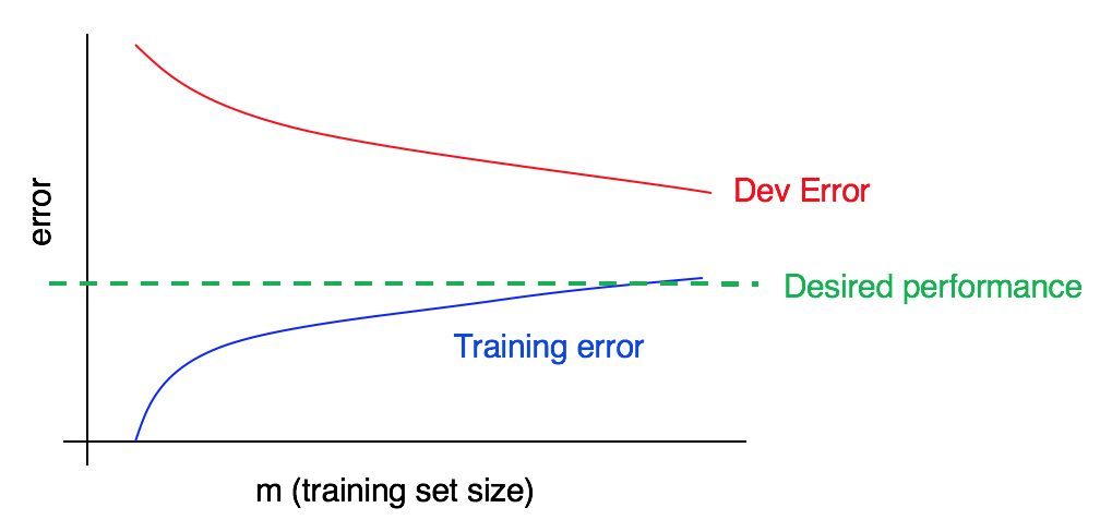
Is this plot indicating, high bias, high variance or both?

The training error is very close to desired performance, indicating avoidable bias is very low. The training(blue) error curve is relatively low, and dev(red) error is much higher than training error. Thus, the bias is small, but variance is large. As from recap above, adding more training data will help close gap between training and dev error and help reduce high variance.

Consider this curve,

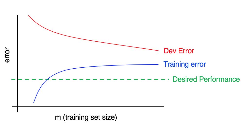
Is this plot indicating, high bias, high variance or both?

This time, training error is large, as it is much higher than desired performance. There is significant avoidable bias. The dev error is also much larger than training error. This indicated we have significant bias and significant variance in our plot. We will use the ways to avoid both variance and bias.

Consider this curve,

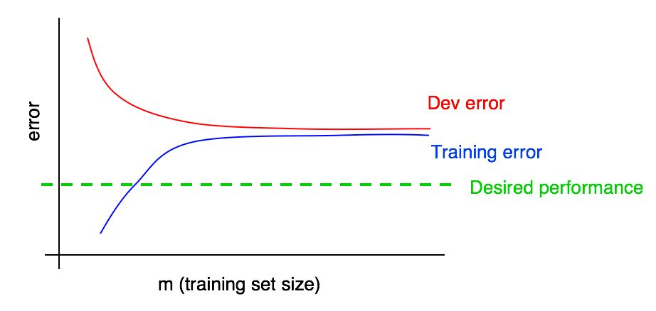
Is this plot indicating, high bias, high variance or both?

The training error is much higher than desired performance. This indicates it has high avoidable bias. The gap between training and dev error curves is small, indicating small variance.

Lessons:

As we add more training data, training error can only get worse. Thus, the blue training error curve can only stay the same or go higher, and thus it can only get further away from the (green line) level of desired performance.
The red dev error curve is usually higher than the blue training error. Thus, there’s almost no way that adding more data would allow the red dev error curve to drop down to the desired level of performance when even the training error is higher than the desired level of performance.

Techniques to reduce avoidable bias

Increase model size (number of neurons/layers)

This technique reduces bias by fitting training set better. If variance increases, we can use regularization to minimize the effect of increase in variance.

Modify input features based on insights from error analysis

Create additional features that help the algorithm eliminate a particular category of errors.These new features could help with both bias and variance.

Reduce or eliminate regularization (L2 regularization, L1 regularization, dropout)

This will reduce avoidable bias, but increase variance.

Modify model architecture (such as neural network architecture)

This technique can affect both bias and variance.

Techniques to reduce variance

Add more training data

This is the simplest and most reliable way to address variance, so long as you have access to significantly more data and enough computational power to process the data.

Add regularization (L2 regularization, L1 regularization, dropout)

This technique reduces variance but increases bias.

Add early stopping (i.e., stop gradient descent early based on dev set error)

This technique reduces variance but increases bias.

Feature selection to decrease number/type of input features

This technique might help with variance problems, but it might also increase bias. Reducing the number of features slightly (say going from 1,000 features to 900) is unlikely to have a huge effect on bias. Reducing it significantly (say going from 1,000 features to 100—a 10x reduction) is more likely to have a significant effect, so long as you are not excluding too many useful features. In modern deep learning, when data is plentiful, there has been a shift away from feature selection, and we are now more likely to give all the features we have to the algorithm and let the algorithm sort out which ones to use based on the data. But when your training set is small, feature selection can be very useful.

Modify model architecture and modify input features

These techniques are also mentioned in avoidable bias.

Data Mismatch

Suppose a ML in a setting where the training and the dev/test distributions are different. Say, the training set contains Internet images + Mobile images, and the dev/test sets contain only Mobile images.

If the model generalizes well to new data drawn from the same distribution as the training set, but not to data drawn from the dev/test set distribution. We call this problem data mismatch , since it is because the training set data is a poor match for the dev/test set data.

This illustration explains clearly the data mismatch problem.

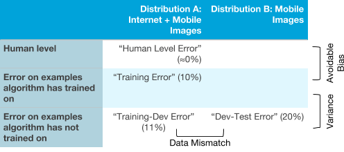
Training set

This is the data that the algorithm will learn from (e.g., Internet images + Mobile images). This does not have to be drawn from the same distribution as what we really care about (the dev/test set distribution).

Training dev set

This data is drawn from the same distribution as the training set (e.g.,Internet images + Mobile images). This is usually smaller than the training set; it only needs to be large enough to evaluate and track the progress of our learning algorithm.

Dev set

This is drawn from the same distribution as the test set, and it reflects the distribution of data that we ultimately care about doing well on. (E.g., mobile images.)

Test set

This is drawn from the same distribution as the dev set. (E.g., mobile images.)

Techniques to resolve data mismatch problem

Try to understand what properties of the data differ between the training and the dev set distributions.
Try to find more training data that better matches the dev set examples that your algorithm has trouble with.

In next post, we will discuss about various regularization techniques and when and how to use them. Stay tuned!

Introduction to Transfer Learning

A long time ago in a galaxy far, far away….

I-know-everything: Yo, my fellow apperentice. This time you will experience the Power of Transfer Learning. Transfer Learning is a technique where you take a pretrained model trained on large dataset and transfer the learned knowledge to another model with small dataset but some what similar to large dataset for task of classification. For e.g. if we consider Imagenet dataset which contains 1.2 million images and 1000 categories, in that there are 24 different categories of dogs and 16 different categories of cats. So, we can transfer the learned features of cats and dogs from model trained on Imagenet dataset to our new model which contains 25,000 images of dogs and cats in training set.

I-know-nothing: Ahh?

I-know-everything: Okay, let’s take a step back and go over our learning from Force of CNN. First, we saw what a convolution operator is, how different kernels or the numbers i n matrix give differnet results when applied to an image such as edge detector, blurring, sharpening, etc. After that, we visited different functions and looked at their properties and role in CNN, e.g. kernel, pooling, strides. We saw CNN consists of multiple CONV-RELU-POOL layers, followed by FC layers like the one shown below.

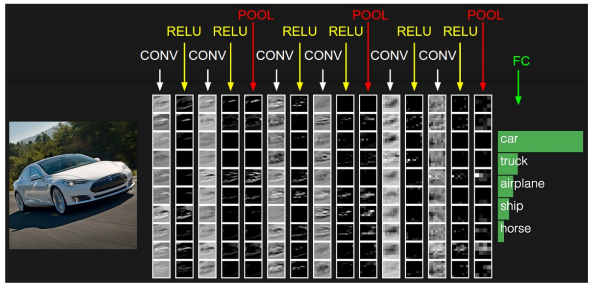
We saw how the training a CNN is similar to MLP. It consists of forward pass followed by backward pass where the kernels adjust the weights so as to backpropagate the error in classification and also looked at different architectures and role they played in Imagenet competition. The only thing we did not discuss is that what these CNN are learning that makes them able to classify 1.2 million images in 1000 categories with 2.25% top5 error rate better than humans. What is going on insides these layers to make them such better classifiers?

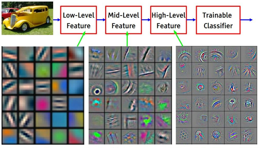
Many details of how these models works is still a mystery (black-box), but Zeiler and Fergus showed in their excellent paper on Visualizaing and Understanding Convolution Neural Networks, that lower convolutional layers capture low-level image features, e.g. edges, while higher convolutional layers capture more and more complex details, such as body parts, faces, and other compositional features.

The final fully-connected layers are generally assumed to capture information that is relevant for solving the respective task, e.g. AlexNet’s fully-connected layers would indicate which features are relevant to classify an image into one of 1000 object categories.

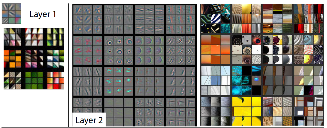
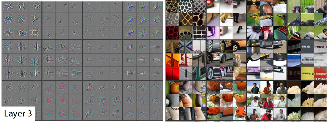
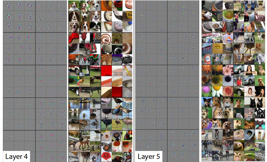
As we observe in above pictures, different layers correspond or activate to different features in the images. For e.g., Layer 3 activates for different textures, Layer 2 activates for different edges and circles, similarly, Layer 5 activates for faces of humans, animals also, they learn to identify text in the image on their own.

In short, here is how CNN learns.

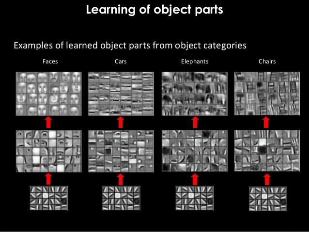
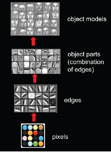
When an image of face of human is passed through CNN, the initial layers learn to identify simple features like nose, eyes, ears, etc. As we move up the architecture, the higher layers will combine simple features into more complex feature and finally dense layers at the top of the network will combine very high level features and produce classification predictions.

I-know-nothing: Now I understand what goes behind the scenes of CNN model. So, how can these features help us in training our model?

I-know-everything: Glad you asked. Transfer learning is an optimization, a shortcut to saving time or getting better performance. There are three possible benefits to look for when using transfer learning:

Higher start: The initial skill (before refining the model) on the source model is higher than it otherwise would be.
Higher slope: The rate of improvement of skill during training of the source model is steeper than it otherwise would be.
Higher asymptote: The converged skill of the trained model is better than it otherwise would be.

On some problems where you may not have very much data, transfer learning can enable you to develop skillful models that you simply could not develop in the absence of transfer learning.

For a new classification task, we can simply use the off-the-shelf features of a state-of-the-art CNN pre-trained on ImageNet and train a new model on these extracted features.

Taking the example of our dataset, where pretrained model has already seen bunch of cats and dogs from Imagenet dataset and now the model is somewhat adept to know difference between cats and dogs and many other different things from Imagenet dataset. So, if we just train the pretrain model with our new dataset of just cats and dogs, the model has already learned how different breeds of dogs and cats looks like. Building on these knowledge of what pretrained model has learned, transferring these to a new model, it learns to classify the images in new dataset very quickly.

2 Major Transfer Learning scenarios

There are 2 major Transfer Learning scenarios:

ConvNet as fixed feature extractor

Take a ConvNet pretrained on ImageNet, remove the last fully-connected layer (this layer’s outputs are the 1000 class scores for a different task like ImageNet), then treat the rest of the ConvNet as a fixed feature extractor for the new dataset. For eg, in AlexNet, this would compute a 4096-D vector for every image that contains the activations of the hidden layer immediately before the classifier. We call these features CNN codes. Once you extract the 4096-D codes for all images, train a linear classifier (e.g. Linear SVM or Softmax classifier) for the new dataset.

In our case of dogs and cats dataset, we will leverage any of the pretrained architectures mentioned in our previous post on CNN, and use them as base model for transfer learning. We will remove the final layer and insert a new hidden layers with desired number of classes for classification as per our new dataset. (or, also we could add multiple different number if hidden layers in between this pretrained model and our output classes) This is one type of transfer learning we can leverage without having to design new architecture and having to worry if it will even work for such smaller dataset(our cats and dogs dataset) or amount of regularization or number of layers or number of neurons in each layer, etc and training on it from scratch. This technique surprisingly gives amazing results in such less time and less compute power than the model trained from scratch will take hours or days of compute power to achieve similar or better results.

Finetuning the ConvNet

The second strategy is to not only replace and retrain the classifier on top of the ConvNet on the new dataset, but to also fine-tune the weights of the pretrained network by continuing the backpropagation. It is possible to fine-tune all the layers of the ConvNet, or it’s possible to keep some of the earlier layers fixed (due to overfitting concerns) and only fine-tune some higher-level portion of the network. This is motivated by the observation that the earlier features of a ConvNet contain more generic features (e.g. edge detectors or color blob detectors) that should be useful to many tasks, but later layers of the ConvNet becomes progressively more specific to the details of the classes contained in the original dataset. In case of ImageNet for example, which contains many dog breeds, a significant portion of the representational power of the ConvNet may be devoted to features that are specific to differentiating between dog breeds.

In our case of dataset, we can use any of pretrained architectures and fine-tune the model by unfreezing last or last 2 convolution blocks depending on size of dataset and compute power avaliable to training. This technique provides a further boost in performance than previous feature extractor technique in orders of magnitutde ranging from 0.5% to 3% but also take significant amount of time to train as we are unfreezing and training some of the convolution blocks of pretrained model.

Next question would be when and how to fine-tune?

This is a function of several factors, but the two most important ones are the size of the new dataset (small or big), and its similarity to the original dataset (e.g. ImageNet-like in terms of the content of images and the classes, or very different, such as microscope images). Keeping in mind that ConvNet features are more generic in early layers and more original-dataset-specific in later layers, here are some common rules of thumb for navigating the 4 major scenarios:

New dataset is small and similar to original dataset

Since the data is small, it is not a good idea to fine-tune the ConvNet due to overfitting concerns. Since the data is similar to the original data, we expect higher-level features in the ConvNet to be relevant to this dataset as well. Hence, the best idea might be to train a linear classifier on the CNN codes.

New dataset is large and similar to the original dataset

Since we have more data, we can have more confidence that we won’t overfit if we were to try to fine-tune through the full network.

New dataset is small but very different from the original dataset

Since the data is small, it is likely best to only train a linear classifier. Since the dataset is very different, it might not be best to train the classifier form the top of the network, which contains more dataset-specific features. Instead, it might work better to train the SVM classifier from activations somewhere earlier in the network.

New dataset is large and very different from the original dataset

Since the dataset is very large, we may expect that we can afford to train a ConvNet from scratch. However, in practice it is very often still beneficial to initialize with weights from a pretrained model. In this case, we would have enough data and confidence to fine-tune through the entire network.

So, my Young Padwan, you have now the full Power of Transfer Learning and we will implement it below. And always remember the wise words spoken by Master Andrej Karpathy, “Don’t be a hero. Instead of rolling your own architecture for a problem, you should look at whatever architecture currently works best on ImageNet, download a pretrained model and finetune it on your data. You should rarely ever have to train a ConvNet from scratch or design one from scratch.” Indeed transfer learning is your go to learning technique whenever images are inputs as long as we have some ConvNet model pretrained on significantly larger dataset which somewhat resemebles or supersets our desired dataset. The performance boost and training time saved by using transfer learning is amazing and must be one of the first methods resorted when inputs are images.

In next post, we will focus on Power to Visualize CNN.

By now you must have a concrete ideas about when to use Sequential and Functional API of any framework. So, we will stick to one such API in our implementation and adding implementation of both frameworks will take a lot of scrolling. Let’s avoid that and use one framework.

Recap

Firstly, we recapped what a CNN is and how a CNN is trained.
Next, we introduce what is transfer learning which led us to thinking about what a CNN learns.
We looked at what the different layers in CNN learns and how we can leverage the same learning by transfer that knowledge to similar tasks.
We looked at different ways to perform transfer learning and how transferring the knowledge helps faster learning. Primarily the two types of transferring learning include, first convnet as feature extractor where a pretrained model (models trained on Imagenet or any bigger datasets) is taken as base model and the last layer in case of Imagenet contains FC layer of 1000 units(neurons) for classifying input image in 1000 categories is cut off(removed) and replaced with our desired number of units(neurons or number of classes) and while training all the layers are frozen except the last layer inserted, and whole model is trained for our new dataset with desired number of classes. And second include, finetuning where we take above architecture and unfreeze some of layers in above frozen layers in pretrained model and retrain the model with same dataset to get new improved performance(better than previous feature extractor).
We looked into different ways to fine-tune a pretrained model and when to fine-tune depending on type of dataset.
We concluded that transfer learning saves a lot of time and energy(electricity unless you are on Googlion planet, to cover your bills) and is one of the best techniques out there to provide state of the art image classification.

Keras

# load all the required libraries

import random
import numpy as np
from tqdm import tqdm
from sklearn.model_selection import train_test_split  # split dataset
import keras                                          # import keras with tensorflow as backend
from keras.preprocessing import image
from keras.preprocessing.image import ImageDataGenerator, array_to_img, load_img, img_to_array
from keras.applications.resnet50 import preprocess_input
from keras.applications.vgg16 import VGG16
from keras.models import Model, Sequential            # sequential and functional api keras 
from keras.layers import Dense, Input, Conv2D, GlobalAveragePooling2D
from keras.layers import Dropout, Flatten, MaxPooling2D, InputLayer # dense and input layer for constructing mlp
from keras.optimizers import SGD
np.random.seed(42)

Using TensorFlow backend.

# # use small subset of train, val and test

train_cats = os.listdir(train_cats_dir)
train_cats = random.sample(train_cats, 2000)
train_dogs = os.listdir(train_dogs_dir)
train_dogs = random.sample(train_dogs, 2000)
val_cats = os.listdir(val_cats_dir)
val_cats = random.sample(val_cats, 400)
val_dogs = os.listdir(val_dogs_dir)
val_dogs = random.sample(val_dogs, 400)
test_img = os.listdir(test_path)
test_img = random.sample(test_img, 50)

print ('New Training set images', len(train_cats)+len(train_dogs))
print ('New Validation set images', len(val_cats)+len(val_dogs))
print ('New Testing set images', len(test_img))

New Training set images 4000
New Validation set images 800
New Testing set images 50

IMG_DIM = (224, 224)

train_X = [train_cats_dir+cats for cats in train_cats]
train_X = train_X + [train_dogs_dir+dogs for dogs in train_dogs]
train_imgs = [img_to_array(load_img(img, target_size=IMG_DIM)) for img in train_X]
train_imgs = np.array(train_imgs)
train_labels = [l.split('/')[-1].split('.')[0].strip('0123456789') for l in train_X]
train_labels = np.array(train_labels)
print ('Training shape:', train_imgs.shape, train_labels.shape) 

val_X = [val_cats_dir+cats for cats in val_cats]
val_X = val_X + [val_dogs_dir+dogs for dogs in val_dogs]
val_imgs = [img_to_array(load_img(img, target_size=IMG_DIM)) for img in val_X]
val_imgs = np.array(val_imgs)
val_labels = [l.split('/')[-1].split('.')[0].strip('0123456789') for l in val_X]
val_labels = np.array(val_labels)
print ('Validation shape:', val_imgs.shape, val_labels.shape) 

test_X = [test_path+imgs for imgs in test_img]
test_X = random.sample(test_X, 50)
test_imgs = [img_to_array(load_img(img, target_size=IMG_DIM)) for img in test_X]
test_imgs = np.array(test_imgs)
print ('Testing shape:', test_imgs.shape) 

Training shape: (4000, 224, 224, 3) (4000,)
Validation shape: (800, 224, 224, 3) (800,)
Testing shape: (50, 224, 224, 3)

# encode text category labels
from sklearn.preprocessing import LabelEncoder

le = LabelEncoder()
le.fit(train_labels)
train_labels_enc = le.transform(train_labels)
val_labels_enc = le.transform(val_labels)

print(train_labels[:5], train_labels_enc[:5])

['cat' 'cat' 'cat' 'cat' 'cat'] [0 0 0 0 0]

Visualization of data

Enough talk, show me the cats and dogs!

def preprocess_img(img, ax, label, train_dir):
    im = Image.open(os.path.join(train_dir, img))
    size = im.size
    ax.imshow(im)
    ax.set_title(f'{label} {size}')

train_x = os.listdir(train_cats_dir)
# plot the images in the batch, along with the corresponding labels
fig = plt.figure(figsize=(25, 10))

for idx in np.arange(10):
    ax = fig.add_subplot(2, 10/2, idx+1, xticks=[], yticks=[])
    preprocess_img(train_x[idx], ax, 'cat', train_cats_dir)
    # print out the correct label for each image

train_x = os.listdir(train_dogs_dir)
# plot the images in the batch, along with the corresponding labels
fig = plt.figure(figsize=(25, 10))

for idx in np.arange(10):
    ax = fig.add_subplot(2, 10/2, idx+1, xticks=[], yticks=[])
    preprocess_img(train_x[idx], ax, 'dog', train_dogs_dir)
    # print out the correct label for each image

ConvNet as feature extractor

# [0-9] unique labels
batch_size = 50
num_classes = 2
epochs = 50

# input image dimensions
img_width, img_height = 224, 224
input_shape = (img_width, img_height, 3)

train_datagen = ImageDataGenerator(rescale=1./255, 
                                   zoom_range=0.3, 
                                   rotation_range=50,
                                   width_shift_range=0.2, 
                                   height_shift_range=0.2, 
                                   shear_range=0.2, 
                                   horizontal_flip=True, 
                                   fill_mode='nearest')

val_datagen = ImageDataGenerator(rescale=1./255)

train_generator = train_datagen.flow(train_imgs, train_labels_enc, batch_size=80)
val_generator = val_datagen.flow(val_imgs, val_labels_enc, batch_size=16)

def pretrained_models(name):
    
    if name == 'VGG16':
        base_model = VGG16(weights='imagenet', include_top=False, pooling='avg')
        for layer in base_model.layers:
          layer.trainable = False
        x = base_model.output

        x = Dense(256, activation='relu')(x)
        x = Dropout(0.5)(x)
        x = Dense(128, activation='relu')(x)
        x = Dropout(0.7)(x)
        output = Dense(1, activation='sigmoid')(x)
        model = Model(inputs=base_model.input, outputs=output)
  
    return model

vgg_model = pretrained_models('VGG16')

vgg_model.trainable = False
for layer in vgg_model.layers:
  layer.trainable = False

import pandas as pd
pd.set_option('max_colwidth', -1)
layers = [(layer.name, layer.trainable) for layer in vgg_model.layers]
pd.DataFrame(layers, columns=['Layer Name', 'Layer Trainable'])  

Downloading data from https://github.com/fchollet/deep-learning-models/releases/download/v0.1/vgg16_weights_tf_dim_ordering_tf_kernels_notop.h5
58892288/58889256 [==============================] - 1s 0us/step

	Layer Name	Layer Trainable
0	input_1	False
1	block1_conv1	False
2	block1_conv2	False
3	block1_pool	False
4	block2_conv1	False
5	block2_conv2	False
6	block2_pool	False
7	block3_conv1	False
8	block3_conv2	False
9	block3_conv3	False
10	block3_pool	False
11	block4_conv1	False
12	block4_conv2	False
13	block4_conv3	False
14	block4_pool	False
15	block5_conv1	False
16	block5_conv2	False
17	block5_conv3	False
18	block5_pool	False
19	flatten_1	False

vgg_model.compile(loss='binary_crossentropy',
              optimizer='Adam',
              metrics=['accuracy'])

es = EarlyStopping(monitor='val_acc', patience=5)

vgg_model.summary()

  Layer (type)                 Output Shape              Param #   
  =================================================================
  input_1 (InputLayer)         (None, None, None, 3)     0         
  _________________________________________________________________
  block1_conv1 (Conv2D)        (None, None, None, 64)    1792      
  _________________________________________________________________
  block1_conv2 (Conv2D)        (None, None, None, 64)    36928     
  _________________________________________________________________
  block1_pool (MaxPooling2D)   (None, None, None, 64)    0         
  _________________________________________________________________
  block2_conv1 (Conv2D)        (None, None, None, 128)   73856     
  _________________________________________________________________
  block2_conv2 (Conv2D)        (None, None, None, 128)   147584    
  _________________________________________________________________
  block2_pool (MaxPooling2D)   (None, None, None, 128)   0         
  _________________________________________________________________
  block3_conv1 (Conv2D)        (None, None, None, 256)   295168    
  _________________________________________________________________
  block3_conv2 (Conv2D)        (None, None, None, 256)   590080    
  _________________________________________________________________
  block3_conv3 (Conv2D)        (None, None, None, 256)   590080    
  _________________________________________________________________
  block3_pool (MaxPooling2D)   (None, None, None, 256)   0         
  _________________________________________________________________
  block4_conv1 (Conv2D)        (None, None, None, 512)   1180160   
  _________________________________________________________________
  block4_conv2 (Conv2D)        (None, None, None, 512)   2359808   
  _________________________________________________________________
  block4_conv3 (Conv2D)        (None, None, None, 512)   2359808   
  _________________________________________________________________
  block4_pool (MaxPooling2D)   (None, None, None, 512)   0         
  _________________________________________________________________
  block5_conv1 (Conv2D)        (None, None, None, 512)   2359808   
  _________________________________________________________________
  block5_conv2 (Conv2D)        (None, None, None, 512)   2359808   
  _________________________________________________________________
  block5_conv3 (Conv2D)        (None, None, None, 512)   2359808   
  _________________________________________________________________
  block5_pool (MaxPooling2D)   (None, None, None, 512)   0         
  _________________________________________________________________
  global_average_pooling2d_1 ( (None, 512)               0         
  _________________________________________________________________
  dense_1 (Dense)              (None, 256)               131328    
  _________________________________________________________________
  dropout_1 (Dropout)          (None, 256)               0         
  _________________________________________________________________
  dense_2 (Dense)              (None, 128)               32896     
  _________________________________________________________________
  dropout_2 (Dropout)          (None, 128)               0         
  _________________________________________________________________
  dense_3 (Dense)              (None, 1)                 129       
  =================================================================
  Total params: 14,879,041
  Trainable params: 164,353
  Non-trainable params: 14,714,688
  _________________________________________________________________

history = vgg_model.fit_generator(train_generator, 
                                  steps_per_epoch=train_generator.n//train_generator.batch_size, 
                                  epochs=50,
                                  validation_data=val_generator, 
                                  validation_steps=val_generator.n//val_generator.batch_size,
                                  callbacks=[es]) 

WARNING:tensorflow:From /usr/local/lib/python3.6/dist-packages/tensorflow/python/ops/math_ops.py:3066: to_int32 (from tensorflow.python.ops.math_ops) is deprecated and will be removed in a future version.
Instructions for updating:
Use tf.cast instead.
Epoch 1/50
50/50 [==============================] - 71s 1s/step - loss: 0.7123 - acc: 0.5368 - val_loss: 0.6182 - val_acc: 0.6913
Epoch 2/50
50/50 [==============================] - 61s 1s/step - loss: 0.5820 - acc: 0.7070 - val_loss: 0.4116 - val_acc: 0.8287
Epoch 3/50
50/50 [==============================] - 62s 1s/step - loss: 0.4497 - acc: 0.7925 - val_loss: 0.3335 - val_acc: 0.8525
Epoch 4/50
50/50 [==============================] - 62s 1s/step - loss: 0.3996 - acc: 0.8243 - val_loss: 0.3250 - val_acc: 0.8550
Epoch 5/50
50/50 [==============================] - 62s 1s/step - loss: 0.3721 - acc: 0.8447 - val_loss: 0.2676 - val_acc: 0.8788
Epoch 6/50
50/50 [==============================] - 61s 1s/step - loss: 0.3405 - acc: 0.8535 - val_loss: 0.2598 - val_acc: 0.8762
Epoch 7/50
50/50 [==============================] - 62s 1s/step - loss: 0.3188 - acc: 0.8615 - val_loss: 0.2539 - val_acc: 0.8838
Epoch 8/50
50/50 [==============================] - 62s 1s/step - loss: 0.3131 - acc: 0.8670 - val_loss: 0.2635 - val_acc: 0.8788
Epoch 9/50
50/50 [==============================] - 62s 1s/step - loss: 0.3080 - acc: 0.8693 - val_loss: 0.2353 - val_acc: 0.8938
Epoch 10/50
50/50 [==============================] - 62s 1s/step - loss: 0.3045 - acc: 0.8675 - val_loss: 0.2404 - val_acc: 0.8912
Epoch 11/50
50/50 [==============================] - 61s 1s/step - loss: 0.2960 - acc: 0.8742 - val_loss: 0.2791 - val_acc: 0.8712
Epoch 12/50
50/50 [==============================] - 61s 1s/step - loss: 0.3042 - acc: 0.8715 - val_loss: 0.2397 - val_acc: 0.8825
Epoch 13/50
50/50 [==============================] - 62s 1s/step - loss: 0.2966 - acc: 0.8760 - val_loss: 0.2435 - val_acc: 0.8825
Epoch 14/50
50/50 [==============================] - 62s 1s/step - loss: 0.2789 - acc: 0.8780 - val_loss: 0.2359 - val_acc: 0.8912

# summarize history for accuracy
plt.plot(history.history['acc'])
plt.plot(history.history['val_acc'])
plt.title('model accuracy')
plt.ylabel('accuracy')
plt.xlabel('epoch')
plt.legend(['train', 'val'], loc='upper left')
plt.show()
# summarize history for loss
plt.plot(history.history['loss'])
plt.plot(history.history['val_loss'])
plt.title('model loss')
plt.ylabel('loss')
plt.xlabel('epoch')
plt.legend(['train', 'val'], loc='upper left')
plt.show()

test_predictions = vgg_model.predict_on_batch(test_imgs/225.)
print (test_predictions.shape)

(50, 1)

# obtain one batch of test images
images, predict = test_imgs, test_predictions

# convert output probabilities to predicted class
preds = (predict > 0.5).astype('int')

# plot the images in the batch, along with predicted and true labels
fig = plt.figure(figsize=(25, 4))
for idx in np.arange(20):
    ax = fig.add_subplot(2, 20/2, idx+1, xticks=[], yticks=[])
    ax.imshow(array_to_img(images[idx]))
    if preds[idx] == 0:
        test_predictions[idx] = 1-test_predictions[idx]
    ax.set_title("{:.2f} % Accuracy {}".format(float(test_predictions[idx][0]*100), 'cat' if preds[idx]==0 else 'dog'))

v_datagen = ImageDataGenerator(rescale=1./255)
val_generator = val_datagen.flow(val_imgs, val_labels_enc, batch_size=batch_size)
img, lbl = val_generator.next()

v_predictions = vgg_model.predict_on_batch(img)
print (v_predictions.shape, lbl.shape)
print (v_predictions[:5], lbl[:5])

(50, 1) (50,)
[[0.5877145 ]
 [1.        ]
 [0.9941321 ]
 [0.98659295]
 [0.00550673]] [1 1 1 1 1]

# obtain one batch of test images
images, predict = img, lbl

# convert output probabilities to predicted class
pred = (predict > 0.5).astype('int')
preds = le.inverse_transform(pred)
labels = le.inverse_transform(lbl)

# plot the images in the batch, along with predicted and true labels
fig = plt.figure(figsize=(25, 4))
for idx in np.arange(20):
    ax = fig.add_subplot(2, 20/2, idx+1, xticks=[], yticks=[])
    ax.imshow(array_to_img(images[idx]))
    ax.set_title("{} ({})".format(str(preds[idx]), str(labels[idx])),
                 color=("green" if preds[idx]==labels[idx] else "red"))

val_preds = vgg_model.predict(val_imgs, batch_size=batch_size)
print (val_preds.shape, val_labels_enc.shape)

(800, 1) (800,)

import scikitplot as skplt

skplt.metrics.plot_confusion_matrix(val_labels_enc, val_preds.astype('int'), normalize=False)

vgg_model.save('bottleneck-features.h5')

Fine tuning

for i, layer in enumerate(vgg_model.layers):
  print (i, layer.name, layer.trainable)

input_1 False
block1_conv1 False
block1_conv2 False
block1_pool False
block2_conv1 False
block2_conv2 False
block2_pool False
block3_conv1 False
block3_conv2 False
block3_conv3 False
block3_pool False
block4_conv1 False
block4_conv2 False
block4_conv3 False
block4_pool False
block5_conv1 False
block5_conv2 False
block5_conv3 False
block5_pool False
global_average_pooling2d_1 False
dense_1 True
dropout_1 True
dense_2 True
dropout_2 True
dense_3 True

# we chose to train the top 1 convolution block, i.e. we will freeze
# the first 15 layers and unfreeze the rest:
for layer in vgg_model.layers[:15]:
    layer.trainable = False
for layer in vgg_model.layers[15:]:
    layer.trainable = True

for i, layer in enumerate(vgg_model.layers):
    print (i, layer.name, layer.trainable)
    
    
vgg_model.compile(loss='binary_crossentropy',
              optimizer=SGD(lr=0.0001, momentum=0.9),
              metrics=['accuracy'])
               
vgg_model.load_weights('bottleneck-features.h5')
  
print (vgg_model.summary())

0 input_1 False
1 block1_conv1 False
2 block1_conv2 False
3 block1_pool False
4 block2_conv1 False
5 block2_conv2 False
6 block2_pool False
7 block3_conv1 False
8 block3_conv2 False
9 block3_conv3 False
10 block3_pool False
11 block4_conv1 False
12 block4_conv2 False
13 block4_conv3 False
14 block4_pool False
15 block5_conv1 True
16 block5_conv2 True
17 block5_conv3 True
18 block5_pool True
19 global_average_pooling2d_1 True
20 dense_1 True
21 dropout_1 True
22 dense_2 True
23 dropout_2 True
24 dense_3 True
_________________________________________________________________
Layer (type)                 Output Shape              Param #   
=================================================================
input_1 (InputLayer)         (None, None, None, 3)     0         
_________________________________________________________________
block1_conv1 (Conv2D)        (None, None, None, 64)    1792      
_________________________________________________________________
block1_conv2 (Conv2D)        (None, None, None, 64)    36928     
_________________________________________________________________
block1_pool (MaxPooling2D)   (None, None, None, 64)    0         
_________________________________________________________________
block2_conv1 (Conv2D)        (None, None, None, 128)   73856     
_________________________________________________________________
block2_conv2 (Conv2D)        (None, None, None, 128)   147584    
_________________________________________________________________
block2_pool (MaxPooling2D)   (None, None, None, 128)   0         
_________________________________________________________________
block3_conv1 (Conv2D)        (None, None, None, 256)   295168    
_________________________________________________________________
block3_conv2 (Conv2D)        (None, None, None, 256)   590080    
_________________________________________________________________
block3_conv3 (Conv2D)        (None, None, None, 256)   590080    
_________________________________________________________________
block3_pool (MaxPooling2D)   (None, None, None, 256)   0         
_________________________________________________________________
block4_conv1 (Conv2D)        (None, None, None, 512)   1180160   
_________________________________________________________________
block4_conv2 (Conv2D)        (None, None, None, 512)   2359808   
_________________________________________________________________
block4_conv3 (Conv2D)        (None, None, None, 512)   2359808   
_________________________________________________________________
block4_pool (MaxPooling2D)   (None, None, None, 512)   0         
_________________________________________________________________
block5_conv1 (Conv2D)        (None, None, None, 512)   2359808   
_________________________________________________________________
block5_conv2 (Conv2D)        (None, None, None, 512)   2359808   
_________________________________________________________________
block5_conv3 (Conv2D)        (None, None, None, 512)   2359808   
_________________________________________________________________
block5_pool (MaxPooling2D)   (None, None, None, 512)   0         
_________________________________________________________________
global_average_pooling2d_1 ( (None, 512)               0         
_________________________________________________________________
dense_1 (Dense)              (None, 256)               131328    
_________________________________________________________________
dropout_1 (Dropout)          (None, 256)               0         
_________________________________________________________________
dense_2 (Dense)              (None, 128)               32896     
_________________________________________________________________
dropout_2 (Dropout)          (None, 128)               0         
_________________________________________________________________
dense_3 (Dense)              (None, 1)                 129       
=================================================================
Total params: 14,879,041
Trainable params: 7,243,777
Non-trainable params: 7,635,264
_________________________________________________________________
None

history = vgg_model.fit_generator(train_generator, 
                                  steps_per_epoch=train_generator.n//train_generator.batch_size, 
                                  epochs=50,
                                  validation_data=val_generator, 
                                  validation_steps=val_generator.n//val_generator.batch_size,
                                  callbacks=[es]) 

 Epoch 1/50
50/50 [==============================] - 68s 1s/step - loss: 0.2812 - acc: 0.8810 - val_loss: 0.2029 - val_acc: 0.9100
Epoch 2/50
50/50 [==============================] - 63s 1s/step - loss: 0.2513 - acc: 0.8965 - val_loss: 0.1999 - val_acc: 0.9000
Epoch 3/50
50/50 [==============================] - 63s 1s/step - loss: 0.2175 - acc: 0.9112 - val_loss: 0.1878 - val_acc: 0.9125
Epoch 4/50
50/50 [==============================] - 63s 1s/step - loss: 0.2150 - acc: 0.9125 - val_loss: 0.1811 - val_acc: 0.9137
Epoch 5/50
50/50 [==============================] - 63s 1s/step - loss: 0.1948 - acc: 0.9187 - val_loss: 0.1746 - val_acc: 0.9212
Epoch 6/50
50/50 [==============================] - 64s 1s/step - loss: 0.1977 - acc: 0.9240 - val_loss: 0.1729 - val_acc: 0.9288
Epoch 7/50
50/50 [==============================] - 63s 1s/step - loss: 0.1911 - acc: 0.9233 - val_loss: 0.1923 - val_acc: 0.9225
Epoch 8/50
50/50 [==============================] - 63s 1s/step - loss: 0.1868 - acc: 0.9257 - val_loss: 0.1797 - val_acc: 0.9275
Epoch 9/50
50/50 [==============================] - 64s 1s/step - loss: 0.1814 - acc: 0.9245 - val_loss: 0.1525 - val_acc: 0.9375
Epoch 10/50
50/50 [==============================] - 63s 1s/step - loss: 0.1612 - acc: 0.9318 - val_loss: 0.1630 - val_acc: 0.9363
Epoch 11/50
50/50 [==============================] - 64s 1s/step - loss: 0.1675 - acc: 0.9362 - val_loss: 0.1660 - val_acc: 0.9337
Epoch 12/50
50/50 [==============================] - 63s 1s/step - loss: 0.1631 - acc: 0.9355 - val_loss: 0.1481 - val_acc: 0.9375
Epoch 13/50
50/50 [==============================] - 63s 1s/step - loss: 0.1648 - acc: 0.9372 - val_loss: 0.1649 - val_acc: 0.9325
Epoch 14/50
50/50 [==============================] - 63s 1s/step - loss: 0.1619 - acc: 0.9320 - val_loss: 0.1361 - val_acc: 0.9437
Epoch 15/50
50/50 [==============================] - 63s 1s/step - loss: 0.1434 - acc: 0.9420 - val_loss: 0.1510 - val_acc: 0.9387
Epoch 16/50
50/50 [==============================] - 64s 1s/step - loss: 0.1511 - acc: 0.9422 - val_loss: 0.1622 - val_acc: 0.9400
Epoch 17/50
50/50 [==============================] - 64s 1s/step - loss: 0.1408 - acc: 0.9487 - val_loss: 0.1432 - val_acc: 0.9500
Epoch 18/50
50/50 [==============================] - 63s 1s/step - loss: 0.1380 - acc: 0.9468 - val_loss: 0.1611 - val_acc: 0.9325
Epoch 19/50
50/50 [==============================] - 64s 1s/step - loss: 0.1381 - acc: 0.9455 - val_loss: 0.1452 - val_acc: 0.9462
Epoch 20/50
50/50 [==============================] - 64s 1s/step - loss: 0.1382 - acc: 0.9460 - val_loss: 0.1416 - val_acc: 0.9437
Epoch 21/50
50/50 [==============================] - 64s 1s/step - loss: 0.1329 - acc: 0.9478 - val_loss: 0.1463 - val_acc: 0.9425
Epoch 22/50
50/50 [==============================] - 64s 1s/step - loss: 0.1270 - acc: 0.9488 - val_loss: 0.1580 - val_acc: 0.9437

# summarize history for accuracy
plt.plot(history.history['acc'])
plt.plot(history.history['val_acc'])
plt.title('model accuracy')
plt.ylabel('accuracy')
plt.xlabel('epoch')
plt.legend(['train', 'val'], loc='upper left')
plt.show()
# summarize history for loss
plt.plot(history.history['loss'])
plt.plot(history.history['val_loss'])
plt.title('model loss')
plt.ylabel('loss')
plt.xlabel('epoch')
plt.legend(['train', 'val'], loc='upper left')
plt.show()

test_predictions = vgg_model.predict_on_batch(test_imgs)
print (test_predictions.shape)

(50, 1)

# obtain one batch of test images
images, predict = test_imgs, test_predictions

# convert output probabilities to predicted class
preds = (predict > 0.5).astype('int')

# plot the images in the batch, along with predicted and true labels
fig = plt.figure(figsize=(25, 4))
for idx in np.arange(20):
    ax = fig.add_subplot(2, 20/2, idx+1, xticks=[], yticks=[])
    ax.imshow(array_to_img(images[idx]))
    if preds[idx] == 0:
        test_predictions[idx] = 1-test_predictions[idx]
    ax.set_title("{:.2f} % Accuracy {}".format(float(test_predictions[idx][0]*100), 'cat' if preds[idx][0]==0 else 'dog'))

vgg_model.save('finetune.h5')

v_datagen = ImageDataGenerator(rescale=1./255)
val_generator = val_datagen.flow(val_imgs, val_labels_enc, batch_size=batch_size)
img, lbl = val_generator.next()

v_predictions = vgg_model.predict_on_batch(img)
print (v_predictions.shape, lbl.shape)
print (v_predictions[:5], lbl[:5])

(50, 1) (50,)
[[8.9467996e-01]
 [3.6521584e-01]
 [4.8128858e-01]
 [1.9999747e-01]
 [5.2365294e-04]] [0 1 1 1 0]

# obtain one batch of test images
images, predict = img, lbl

# convert output probabilities to predicted class
pred = (predict > 0.5).astype('int')
preds = le.inverse_transform(pred)
labels = le.inverse_transform(lbl)

# plot the images in the batch, along with predicted and true labels
fig = plt.figure(figsize=(25, 4))
for idx in np.arange(20):
    ax = fig.add_subplot(2, 20/2, idx+1, xticks=[], yticks=[])
    ax.imshow(array_to_img(images[idx]))
    ax.set_title("{} ({})".format(str(preds[idx]), str(labels[idx])),
                 color=("green" if preds[idx]==labels[idx] else "red"))

val_preds = vgg_model.predict(val_imgs, batch_size=batch_size)
print (val_preds.shape, val_labels_enc.shape)

(800, 1) (800,)

import scikitplot as skplt

skplt.metrics.plot_confusion_matrix(val_labels_enc, val_preds.astype('int'), normalize=False)

I-know-everything: Young Padwan, now that you have seen how Transfer Learning works. The applications of using this approach are limitless, play with everything you can using these pretrained models. In next post, we will visualize layers in CNN and see what parts of image are they looking at. Visualization of layers in CNN plays a crucial role in seeing what is going inside the black box of CNN. Some of the popular visualization techniques include: