Visualizing CNN

In this post, we will try to answer the question “What CNN sees?” using Cats vs Dogs Redux Competition dataset from kaggle. We will implement this using one of the popular deep learning framework Keras .

All the codes implemented in Jupyter notebook in Keras and fastai.

All codes can be run on Google Colab (link provided in notebook). Awesome Tensorflow Library by PAIR Initiative, Lucid by Tensorflow, Keras Vis Library and PyTorch. Try to use libraries instead of writing all the code from scratch. Not that it is bad practise. But we can see the same thing by standing on the the shoulder of giants (less work!).

Hey yo, but how to see what a CNN sees?

Well sit tight and buckle up. I will go through everything in-detail.

Feel free to jump anywhere,

Regularization
- Why does Regularization Work?
- Tips for using Weight Regularization
Introduction to Visualizing CNN
Further Reading
Footnotes and Credits

Regularization

Regualarization, is that another one of the fancy names, to look cooler? After introducing the bias and variance, overfitting and underfitting, ways of interpreting learning curves, now comes the time put all these pieces together. We learned to interpret if our model is overfitting or underfitting from learning curves in our last post on Transfer Learning. So, now we will look into ways of how to handle these anomalies. First, why to use regularizations? All along in machine learning, we tried to make an algorithm that does good not only on training data, but also on new inputs i.e. to generalize data other than training or the unseen data.

If you suspect the model is overfitting (high variance), we call in regularization to rescue. We looked other ways we can do, like adding more data, which is not always the case as it can be expensive to get more data, and so on. So, adding regularization often helps in reducing overfitting (reduce variance). Good regularizers reduces variance significantly while not overly increasing bias.

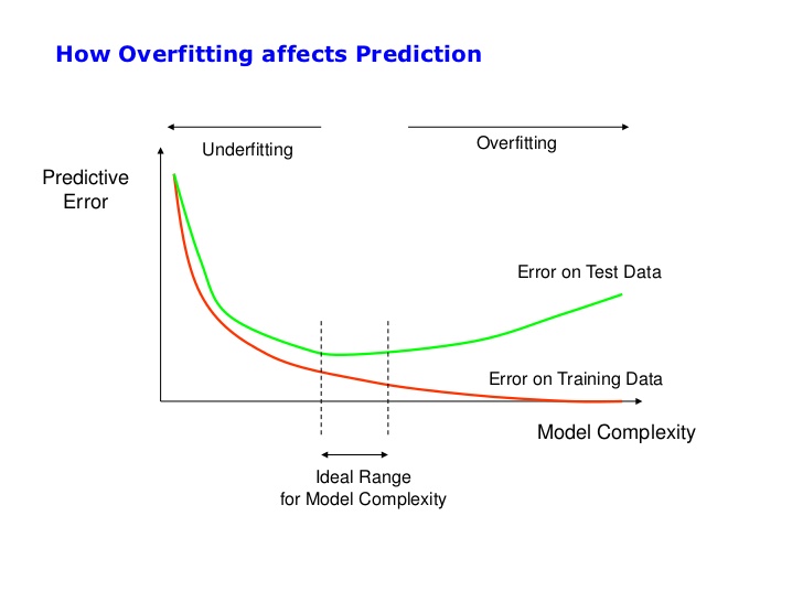
Michael Neilsen explains clearly the relation between parameters in model and generalizability,

Models with a large number of free parameters can describe an amazingly wide range of phenomena. Even if such a model agrees well with the available data, that doesn’t make it a good model. It may just mean there’s enough freedom in the model that it can describe almost any data set of the given size, without capturing any genuine insights into the underlying phenomenon. When that happens the model will work well for the existing data, but will fail to generalize to new situations. The true test of a model is its ability to make predictions in situations it hasn’t been exposed to before.

Here we will dive deep into two well-know regularizers (\(L^1\) and \(L^2\)) and in next post discuss the remaining ones.

\(L^2\) regularization: This regularization goes by many names, Ridge regression, Tikhonov regularization, Weight Decay or Fobenius Norm (used in different contexts). This method imposes a penalty by adding a regularization term \(\Omega(\theta) = \lambda \left\Vert\left(\mathbf{w}\rm\right) \right\Vert^2\) to the objective(loss) function. Here, \(\lambda\) is the regularization parameter. It is the hyperparameter whose value is optimized for better results. The penalty tends to drive all the weights to smaller values.

From Michael Neilsen on \(L^2\) regularization,

Intuitively, the effect of regularization is to make it so the network prefers to learn small weights, all other things being equal. Large weights will only be allowed if they considerably improve the first part of the cost (loss or objective) function. Put another way, regularization can be viewed as a way of compromising between finding small weights and minimizing the original cost function. The relative importance of the two elements of the compromise depends on the value of \(\lambda\): when \(\lambda\) is small we prefer to minimize the original cost function, but when \(\lambda\) is large we prefer small weights.

\(L^1\) regularization: This regularization goes by one other name, LASSO regression (least absolute shrinkage and selection operator). This method imposes a penalty by adding a regularization term \(\Omega(\theta) = \lambda ||\mathbf{w}||\) to the objective(loss) function. Here, \(\lambda\) is the regularization parameter. It is the hyperparameter whose value is optimized for better results. The penalty tends to drive some weights to exactly zero (introducing sparsity in the model), while allowing some weights to be big. The key difference between these techniques is that LASSO shrinks the less important feature’s coefficient to zero thus, removing some feature altogether. So, this works well for feature selection in case we have a huge number of features.

Why does Regularization Work?

Now, the answer question which follows what is, is why? Why does it work? Consider an example below,

Our goal is to build a model that lets us predict \(\mathbf{y}\) as function of \(\mathbf{x}\). First we will fit a polynomial model and then look into case of fitting neural networks. As there are 5 points in graph above, which means we can find a unique 4th-order polynomial \(\mathbf{y}=\mathbf{a_0}+\mathbf{a_1}\mathbf{x_1}+…+\mathbf{a_4}\mathbf{x_4}\) which fits the data exactly as shown in the graph(rightmost). But we can also get a good fit using the quadratic model \(\mathbf{y}=\mathbf{a_0}+\mathbf{a_1}\mathbf{x_1}+\mathbf{a_2}\mathbf{x_2}\), as shown in graph(middle).

Now question is Which of these is the better model? Which is more likely to be true? And which model is more likely to generalize well to other examples of the same underlying real-world phenomenon?

It’s not a priori possible to say which of these two possibilities is correct. (Or, indeed, if some third possibility holds). Logically, either could be true. And it’s not a trivial difference. It’s true that on the data provided there’s only a small difference between the two models. But suppose we want to predict the value of y corresponding to some large value of x, much larger than any shown on the graph above. If we try to do that there will be a dramatic difference between the predictions of the two models.

One point of view is to say that in science we should go with the simpler explanation, unless compelled not to. When we find a simple model that seems to explain many data points we are tempted to shout “Eureka!” After all, it seems unlikely that a simple explanation should occur merely by coincidence. Rather, we suspect that the model must be expressing some underlying truth about the phenomenon.

And so while the 4th order model works perfectly for these particular data points, the model will fail to generalize to other data points, and the noisy 2nd order model will have greater predictive power.

Let’s see what this point of view means for neural networks. Suppose our network mostly has small weights, as will tend to happen in a regularized network. The smallness of the weights means that the behaviour of the network won’t change too much if we change a few random inputs here and there. That makes it difficult for a regularized network to learn the effects of local noise in the data. Think of it as a way of making it so single pieces of evidence don’t matter too much to the output of the network. Instead, a regularized network learns to respond to types of evidence which are seen often across the training set. By contrast, a network with large weights may change its behaviour quite a bit in response to small changes in the input. And so an unregularized network can use large weights to learn a complex model that carries a lot of information about the noise in the training data. In a nutshell, regularized networks are constrained to build relatively simple models based on patterns seen often in the training data, and are resistant to learning peculiarities of the noise in the training data. The hope is that this will force our networks to do real learning about the phenomenon at hand, and to generalize better from what they learn.

Michael Neilsen explains in his book concludes that, “Regularization may give us a computational magic wand that helps our networks generalize better, but it doesn’t give us a principled understanding of how generalization works, nor of what the best approach is.”

Here is an example from the book to understand the above statement,

A network with 100 hidden neurons has nearly 80,000 parameters. We have only 50,000 images in our MNSIT training data. It’s like trying to fit an 80,000th degree polynomial to 50,000 data points. By all rights, our network should overfit terribly. And yet, as we saw earlier, such a network actually does a pretty good job generalizing. Why is that the case? It’s not well understood. It has been conjectured that “the dynamics of gradient descent learning in multilayer nets has a ‘self-regularization’ effect”. This is exceptionally fortunate, but it’s also somewhat disquieting that we don’t understand why it’s the case. In the meantime, we will adopt the pragmatic approach and use regularization whenever we can. Our neural networks will be the better for it.

Tips for using Weight Regularization

Use with All Network Types

Weight regularization is generic technique. It can be used with all types neural networks we saw uptil now, MLP, CNN, LSTM and RNN (which we will address in later posts).

Standardize Input Data

It is generally good practice to update input variables to have the same scale. When input variables have different scales, the scale of the weights of the network will, in turn, vary accordingly. This introduces a problem when using weight regularization because the absolute or squared values of the weights must be added for use in the penalty. This problem can be addressed by either normalizing or standardizing input variables.

Use Larger Network

It is common for larger networks (more layers or more nodes) to more easily overfit the training data. When using weight regularization, it is possible to use larger networks with less risk of overfitting. A good configuration strategy may be to start with larger networks and use weight decay.

Grid Search Parameters

It is common to use small values for the regularization hyperparameter that controls the contribution of each weight to the penalty. Perhaps start by testing values on a log scale, such as 0.1, 0.001, and 0.0001. Then use a grid search at the order of magnitude that shows the most promise.

Use L1 + L2 Together

Rather than trying to choose between L1 and L2 penalties, use both. Modern and effective linear regression methods such as the Elastic Net use both L1 and L2 penalties at the same time and this can be a useful approach to try. This gives you both the nuance of L2 and the sparsity encouraged by L1.

Use on a Trained Network

The use of weight regularization may allow more elaborate training schemes. For example, a model may be fit on training data first without any regularization, then updated later with the use of a weight penalty to reduce the size of the weights of the already well-performing model.

In next post, we will discuss about other regularization techniques and when and how to use them. Stay tuned!

Introduction to Visualizing CNN

A long time ago in a galaxy far, far away….

I-know-everything: Today will be the exiciting topic of peeking inside of the black box of CNNs and look at what they see. So, to recap, from our previous posts we saw what a CNN is, wherein we trained CNN and looked at different architectures. Next, we moved to transfer learning. There we learned what an amazing technique transfer learning is! Different ways of transfer learning and how and why transfer learning provides such a boost. In that topic, we introduced to this notion of CNN as black box, where we really can’t tell as to what is that network is looking at while training or predicting and how such amazing CNN learn to classify 1000 categories of 1.2 million images better than humans. So, today we will look behind the scenes of working of CNNs and this will involve looking at lots of pictures.

Story

Before that let me tell you a story, once upon a time US Army wanted to use neural networks to automatically detect camouflaged enemy tanks. The dataset that reasearchers collected comprised of 50 photos of camouflaged tanks in trees, and 50 photos of trees without tanks. Using standard techniques of supervisied learning, the reasearchers trained a neural network on the given dataset and achieved an output “yes” for the 50 photos of camouflaged tanks, and output “no” for the 50 photos of forest. The researchers handed the finished work to the Pentagon, which soon handed it back, complaining that in their own tests the neural network did no better than chance at discriminating photos. It turned out that in the researchers’ dataset, photos of camouflaged tanks had been taken on cloudy days, while photos of plain forest had been taken on sunny days. The neural network had learned to distinguish cloudy days from sunny days, instead of distinguishing camouflaged tanks from empty forest. Haha! The military was now the proud owner of a multi-million dollar mainframe computer that could tell you if it was sunny or not. How much of this urban legend is true or false is compiled in this blog. Whether happened or not, it sure is a cautionary tale to remind us, to look deep into how neural networks comes to particular conclusion. Trust, but verfify!

I-know-nothing: Ayye Master, I am ready!

I-know-everything: Before jumping to lots of image, let’s look at the architecture that was used in training our model.

  _________________________________________________________________
  Layer (type)                 Output Shape              Param #   
  =================================================================
  input_2 (InputLayer)         (None, 224, 224, 3)       0         
  _________________________________________________________________
  block1_conv1 (Conv2D)        (None, 224, 224, 64)      1792      
  _________________________________________________________________
  block1_conv2 (Conv2D)        (None, 224, 224, 64)      36928     
  _________________________________________________________________
  block1_pool (MaxPooling2D)   (None, 112, 112, 64)      0         
  _________________________________________________________________
  block2_conv1 (Conv2D)        (None, 112, 112, 128)     73856     
  _________________________________________________________________
  block2_conv2 (Conv2D)        (None, 112, 112, 128)     147584    
  _________________________________________________________________
  block2_pool (MaxPooling2D)   (None, 56, 56, 128)       0         
  _________________________________________________________________
  block3_conv1 (Conv2D)        (None, 56, 56, 256)       295168    
  _________________________________________________________________
  block3_conv2 (Conv2D)        (None, 56, 56, 256)       590080    
  _________________________________________________________________
  block3_conv3 (Conv2D)        (None, 56, 56, 256)       590080    
  _________________________________________________________________
  block3_pool (MaxPooling2D)   (None, 28, 28, 256)       0         
  _________________________________________________________________
  block4_conv1 (Conv2D)        (None, 28, 28, 512)       1180160   
  _________________________________________________________________
  block4_conv2 (Conv2D)        (None, 28, 28, 512)       2359808   
  _________________________________________________________________
  block4_conv3 (Conv2D)        (None, 28, 28, 512)       2359808   
  _________________________________________________________________
  block4_pool (MaxPooling2D)   (None, 14, 14, 512)       0         
  _________________________________________________________________
  block5_conv1 (Conv2D)        (None, 14, 14, 512)       2359808   
  _________________________________________________________________
  block5_conv2 (Conv2D)        (None, 14, 14, 512)       2359808   
  _________________________________________________________________
  block5_conv3 (Conv2D)        (None, 14, 14, 512)       2359808   
  _________________________________________________________________
  block5_pool (MaxPooling2D)   (None, 7, 7, 512)         0         
  _________________________________________________________________
  flatten_2 (Flatten)          (None, 25088)             0         
  _________________________________________________________________
  dense_10 (Dense)             (None, 512)               12845568  
  _________________________________________________________________
  dropout_7 (Dropout)          (None, 512)               0         
  _________________________________________________________________
  dense_11 (Dense)             (None, 512)               262656    
  _________________________________________________________________
  dropout_8 (Dropout)          (None, 512)               0         
  _________________________________________________________________
  dense_12 (Dense)             (None, 2)                 1026      
  =================================================================
  Total params: 27,823,938
  Trainable params: 20,188,674
  Non-trainable params: 7,635,264
  _________________________________________________________________

So, it’s VGG16 with last fully connected removed with addition of new FC layers along with dropout.

To start with visualization, we will take a random sample image from our cats and dogs dataset graciously provided by Kaggle. How does these look?

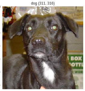
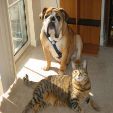
So, we will perform all sorts of not evil experiments on this dog and cats images, using our trained model from transfer learning, we will look at various techniques used for visualizing CNNs.

Visualizing Activations

In this approach, we look at different filter from our model. From our above architecture, we look at block1_conv1, block2_conv1, block3_conv1, block4_conv1, block5_conv1 and block5_conv3 layers(filters). In each layer, some neurons will remain dark while others will light up as they respond to different patterns in the image.

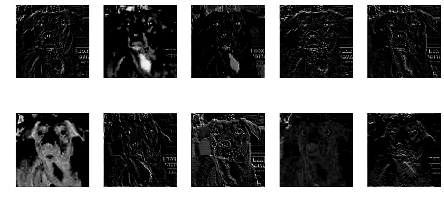
block1_conv1

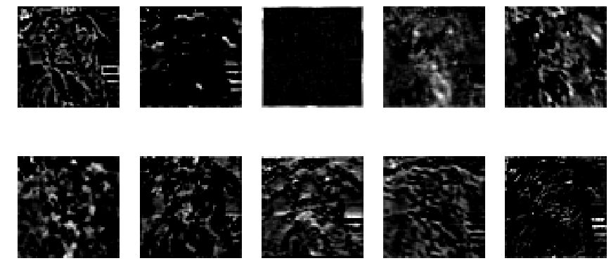
block3_conv1

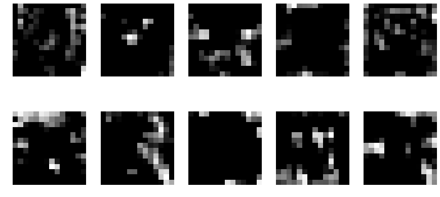
block5_conv1

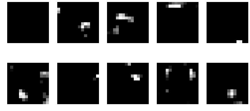
block5_conv3

Well, this black and white isn’t telling much. Let’s apply these as a mask to our original image.

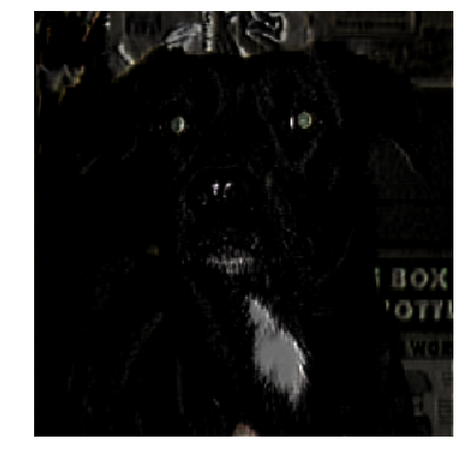
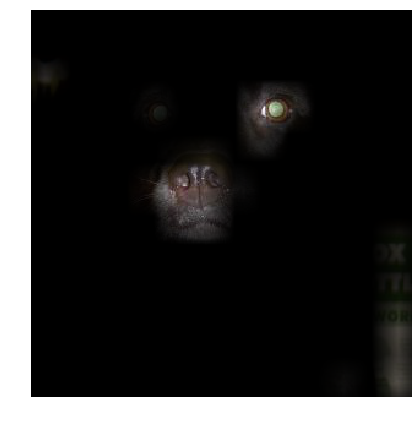
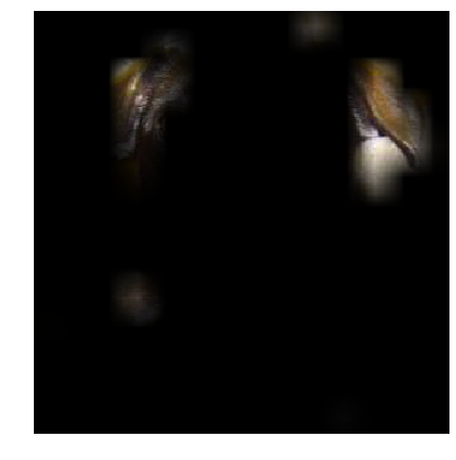
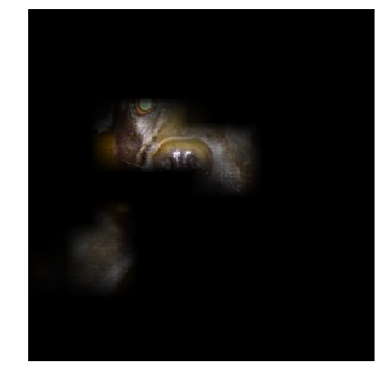
And voila! Wow! We get some amazing results. We see that there are some individual neurons in the filters which look for whiskers and nose of dog, some on left eye, eyes and nose detector and also ears, etc.

Visualize inputs that maximize the activation of the filters in different layers of the model

In this approach, we take our trained model and reconstruct the images that maximize the activation of filters in different layers of the model. The reasoning behind this idea is that a pattern to which the unit is responding maximally could be a good first-order representation of what a unit is doing. One simple way of doing this is to find, for a given unit, the input sample(s) (from either the training or the test set) that give rise to the highest activation of the unit. Here, we take our model and layer name for which pattern is to be discerned. Next, we compute the gradient of input image(random noise) with respect to loss function which maximises the activation of provided layer name. We perform a gradient ascent in the input space with regard to our filter activation loss. This along with some tricks like normalizing input, we get beautiful pattern of what pattern that layer activates most for. We could use the same code to display what sorts of input maximizes each filter in each layer. As there are 100s of filters in some layer, we choose the ones with highest activation to form a grid of 8x8.

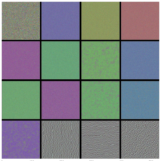
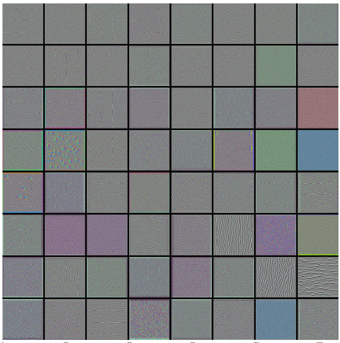
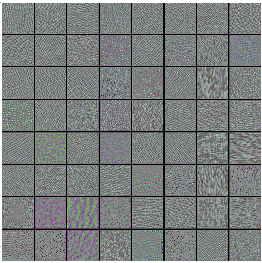
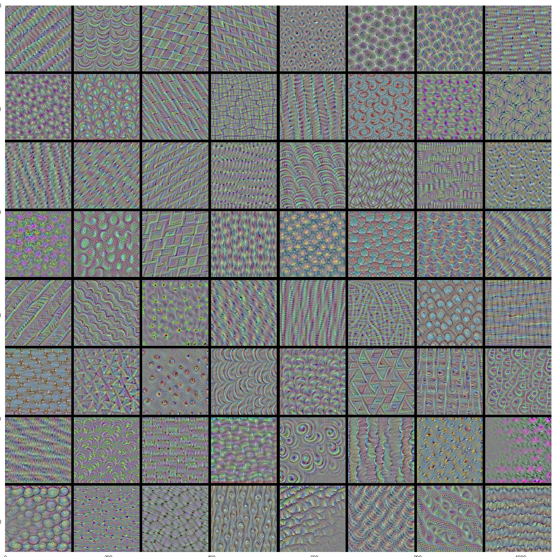
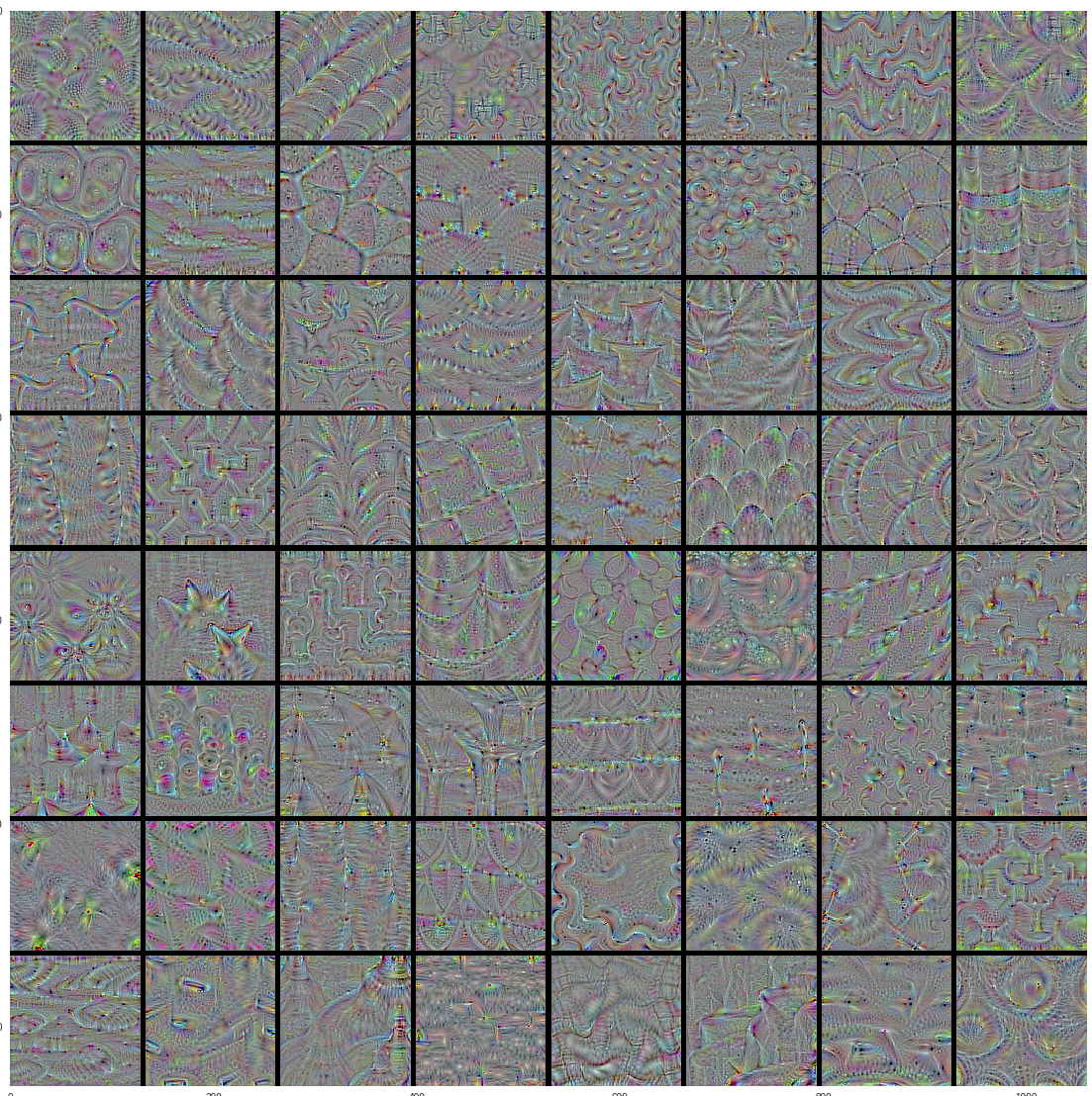
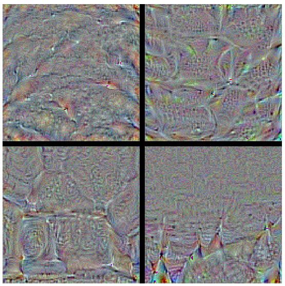
Here are high-res quality images of above visualizations.

We get to see some interesting patterns. The first layers basically just encode direction and color. These direction and color filters then get combined into basic grid and spot textures. These textures gradually get combined into increasingly complex patterns. In the highest layers (block5_conv2, block5_conv3) we start to recognize textures. We confirm our claim from previous post on transfer learning, that the lower convolutional layers capture low-level image features, e.g. edges, while higher convolutional layers capture more and more complex details, such as body parts, faces, and other compositional features. We see that this is indeed the case.

Vanilla Backprop

This is one of the simplest of techniques where we measure the relative importance of input features by calculating the gradient of the output decision with respect to those input features. It simply means that we use the techniques used above like loss function and calculate the gradients of last layer with respect to model input. The image will we somewhat indiscernible but it shows us what part of image it focuses on to make the output decision.

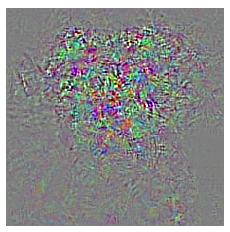
Vanilla Backprop

Guided Backprop

This method is lot like the one above with the only difference was how to handle the backpropagation of gradients through non-linear layers like ReLU. GuidedBackprop, suppressed the flow of gradients through neurons wherein either of input or incoming gradients were negative. Also, Guided Backpropagation visualizations are generally less noisy. The following illustrations explains clearly this phenomenon.

Image Credits

Here is our result,

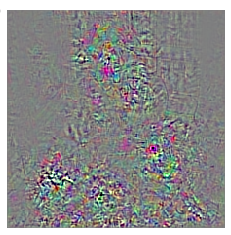
Guided Backprop of only dog image

Grad CAM

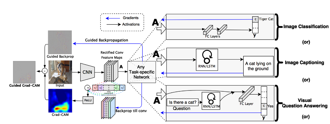
Grad-CAM, uses the gradients of any target concept (say logits for ‘dog’), flowing into the final convolutional layer to produce a coarse localization map highlighting the important regions in the image for predicting the concept. Given an image and a class of interest (‘dog’) as input, we forward propagate the image through the CNN part of the model and then through task-specific computations to obtain a raw score for the category. The gradients are set to zero for all classes except the desired class (dog), which is set to 1. This signal is then backpropagated to the rectified convolutional feature maps of interest, which we combine to compute the coarse Grad-CAM localization (blue heatmap) which represents where the model has to look to make the particular decision. Here is the illustration from original paper.

Image Credits

Here is the result,

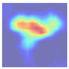
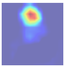
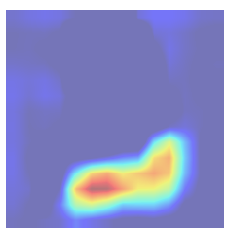
Amazing right? It tells us exactly what region in the input image it has looked at to make the decision of predicting particular class.

Guided Grad CAM

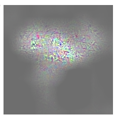
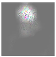
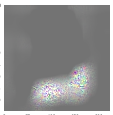
Combining Guided Backprop and Grad CAM from above gives Guided Grad-CAM, which gives high-resolution class-discriminative visualizations. It’s just pointwise multiplication of above two results.

An input that maximizes a specific class

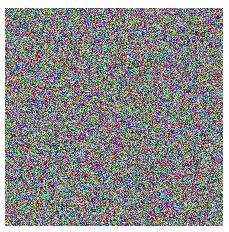
In this method, we take random noise and with choosing a particular class either cat or dog, we construct an input from random noise such that it gives near perfect accurate prediction of chosen class.

Here is the noise,

Noise

This is what we obtain as an image.

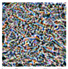
Noise

This is the output predictions when we pass the image through our model. It is almost certain 99.99% sure that this is dog.(Haha! Well, I don’t see how this is a dog.)

array([[1.7701734e-07, 9.9999988e-01]], dtype=float32)

Fchollet on keras blog explains,

So our convnet’s notion of a dog looks nothing like a dog –at best, the only resemblance is at the level of local textures (ears, maybe whiskers or nose). Does it mean that convnets are bad tools? Of course not, they serve their purpose just fine. What it means is that we should refrain from our natural tendency to anthropomorphize them and believe that they “understand”, say, the concept of dog, or the appearance of a magpie, just because they are able to classify these objects with high accuracy. They don’t, at least not to any any extent that would make sense to us humans. So what do they really “understand”? Two things: first, they understand a decomposition of their visual input space as a hierarchical-modular network of convolution filters, and second, they understand a probabilitistic mapping between certain combinations of these filters and a set of arbitrary labels. Naturally, this does not qualify as “seeing” in any human sense, and from a scientific perspective it certainly doesn’t mean that we somehow solved computer vision at this point.

Deep Dream

This is certainly the coolest technique. It’s like our neural network is dreaming. In usual CNN training what we do is adjust the network’s weight to agree more with the image. But here, we instead adjust the image to agree more with the network. If we adjust the image like this, adjusting the pixels a bit at a time and then repeating, then we would actually start to see dogs in the photo, even if there weren’t dogs there to begin with! In other words, instead of forcing the network to generate pictures of dogs or other specific objects, we let the network create more of whatever it saw in the image.

Here is the excerpt from the blog

Instead of exactly prescribing which feature we want the network to amplify, we can also let the network make that decision. In this case we simply feed the network an arbitrary image or photo and let the network analyze the picture. We then pick a layer and ask the network to enhance whatever it detected. Each layer of the network deals with features at a different level of abstraction, so the complexity of features we generate depends on which layer we choose to enhance. For example, lower layers tend to produce strokes or simple ornament-like patterns, because those layers are sensitive to basic features such as edges and their orientations.

If we choose higher-level layers, which identify more sophisticated features in images, complex features or even whole objects tend to emerge. Again, we just start with an existing image and give it to our neural net. We ask the network: “Whatever you see there, I want more of it!” This creates a feedback loop: if a cloud looks a little bit like a bird, the network will make it look more like a bird. This in turn will make the network recognize the bird even more strongly on the next pass and so forth, until a highly detailed bird appears, seemingly out of nowhere.

Here is sample input image,

Cinque Terre Credits

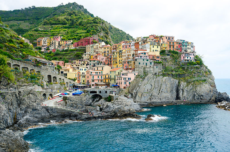
This is the output we obtain,

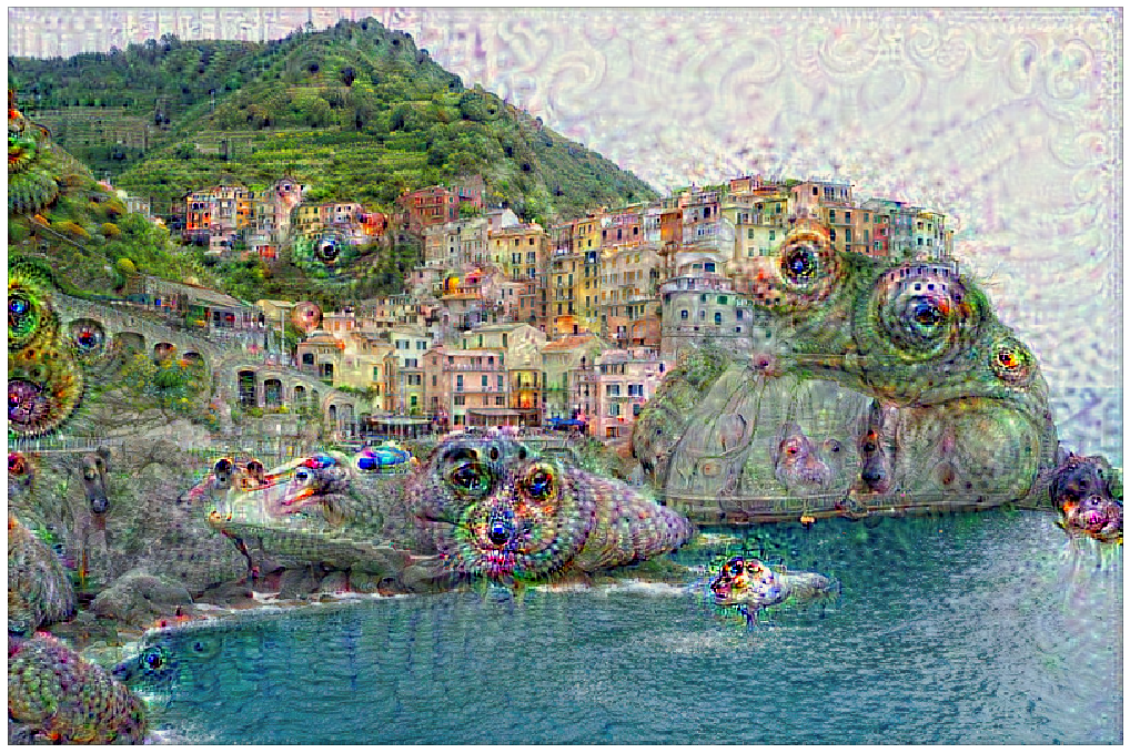
Deep Dream Cinque Terre

We can see lots of dogs in this image. For more deep dreaming, check these results .

t-SNE Visualization

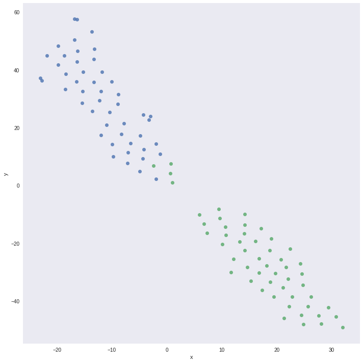
We randomly sample 100 images from training set and use penultimate layer as predictor and visualize these 100 images in embedding projector by Tensorflow. We can visualize these emeddings on the projector along with labels.

We convert the predictons of the penultimate layer from 512 dimension to 2 dimension using t-SNE and plot using corresponding labels. We get the following plots for Perplexity of 15 and 25.

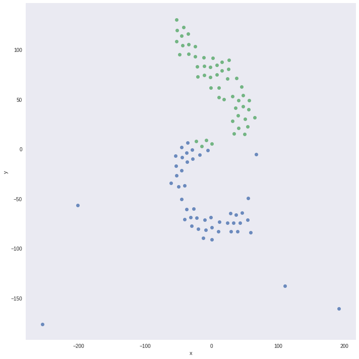
Perplexity 15

Perplexity 25

It shows a clear seperation boundary between the classes of cats and dogs and also shows some missclassified data points.

What we saw above are gradient-based (optimization-based) algorithms, there are also perturbation based techniques and Relevance score based to visualize and interpret the decisions made by deep learning models. The perturbation based techniques include heatmap via occlusion, integrated gradients, super-pixel perturbation, etc.

What a fun ride through the internals of models! Next, we experience the Magic of Style Transfer. You will be suprised what we can achieve with this technique.

Happy Learning!