Neural Style Transfer
In this post, we will try to answer the question “Can we paint as good as Master Picasso?”
All the codes implemented in Jupyter notebook in Keras, PyTorch and fastai.
All codes can be run on Google Colab (link provided in notebook).
Hey yo, but how?
Well sit tight and buckle up. I will go through everything in-detail.
Feel free to jump anywhere,
Regularization
In our previous post to introduction to regularization, we explained why regularization is necessary and gave a brief account of two techniques, \(L^{1}\) and \(L^{2}\) regularizations. We will give a short introduction to remaining techniques. Regualarization techniques are used to control overfitting of the neural network models.
Batch Normalization
We have seen that normalizing input features, aka feature scaling can speed up the training. But once the normalized input is fed to the deep network, as each layer is affected by parameters in all the input layer, even a small change in the network parameter is amplified and leads to the input distribution being changed in the internal layers of the network. This is known as internal covariance shift. Batch Normalization is an idea introduced in excellent paper by (Ioffe & Szegedy) of normalizing activations of every fully connected and convolution layer with unit standard deviation and zero mean during training, as a part of the network architecture itself. Batch Normalization makes the distribution more stable of activation values throughout training and reduces the internal covariance shift in deep networks. It allows us to use much higher learning rates and be less careful about network initialization. It also makes neural networks more robust and can very easily help in training deep networks.
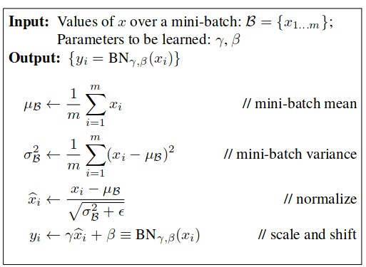
It is implemented as a layer (with trainable parameters) and normalizes the activations of the previous layer. Backpropagation allows the network to learn if they want the activations to be normalized and upto what extent. In practice, batch norm is inserted immediately after fully connected or convolutional layers and before nonlinearities.
More curious audience: Check this recent paper on Batchnorm
Dropout
The key idea is to randomly drop units (along with their connections) from the neural network during training. By dropping a unit out means temporarily removing it from the network, along with all its incoming and outgoing connection as shown below. The choice of which units to drop is random.
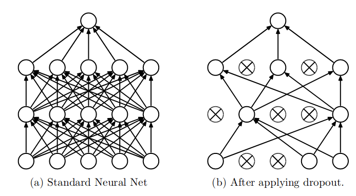
It helps reducing interdependent learning amongst the neurons. Heuristically, when we dropout different sets of neurons, it’s rather like we’re training different neural networks. And so the dropout procedure is like averaging the effects of a very large number of different networks. While training, dropout is implemented by only keeping a neuron active with some probability p (a hyperparameter), or setting it to zero otherwise. During testing there is no dropout applied.

Curious Readers: Did you know?
Data Augmentation
The best way to make a machine learning model generalize better is to train it on more data. Of course, in practice, the amount of data we have is limited. One way to get around this problem is to create fake data and add it to the training set. With more data, come greater capacity of model to learn examples from.
The general principle is to expand the training data by applying operations that reflect real-world variation. There are many ways to augment the data like random crop, center crop, scale, resize, color normalization, contrast, brightness, random zoom, horizontal flip, vertical flip, adding gaussian noise, etc. We are making our neural network more robust to different kinds of real-world scenarios that can occur other than our ideal dataset. One must be careful not to apply transformations that would change the correct class. For example, optical character recognition tasks require recognizing the difference between “b” and “d” and the difference between “6” and “9,” so horizontal flips and 180 degree rotations are not appropriate ways of augmenting datasets for these tasks.
Early Stopping
The idea of Early Stopping is very simple yet effective. Consider below training and validation graph, let us measure the performance of our model on a separate validation dataset during the training iterations. We may then observe that, despite constant score improvements on the training data, the model’s performance on the validation dataset would only improve during the first stage of training, reach an optimum at some point and then turn to getting worse with further iterations. It thus seems reasonable to stop training at the point when the minimal validation error is achieved. Training the model any further only leads to overfitting. Early stopping actually more explicitly limits the complexity of the final model.
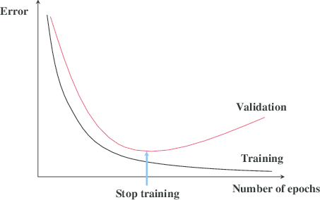
This means we can obtain a model with better validation set error (and thus, hopefully better test set error) by returning to the parameter setting at the point in time with the lowest validation set error. Every time the error on the validation set improves, we store a copy of the model parameters. When the training algorithm terminates, we return these parameters, rather than the latest parameters. The algorithm terminates when no parameters have improved over the best recorded validation error for some pre-specified number of iterations.
In next post, we will discuss some popular loss functions and where are they used. Stay tuned!
Introduction to Neural Style Transfer
A long time ago in a galaxy far, far away….
I-know-everything: Today we will do something creative. We will paint (not literally). To do this we will make use of two of our old powers (Feel the power, Apperentice), Power of Transfer Learning and Force of CNNs. I hope you have practised with your powers well enough! Also, in previous post, we encountered how CNN networks were dreaming (hallucinating) and what are they looking at and how they learn.
I-know-nothing: Does this mean that we will paint as good as Master Picasso?
I-know-everything: Haha, I will let you be the judge of that. It’s fascinating how these algorithms work and the results they produce. I will directly start with multiple ways of how we can achieve such startling results.
Artistic Style Transfer
The excellent paper in 2015 by Gatys et al proposed a neural algorithm that creates artistic images of high perceptual quality. Let’s breakdown how the algorithm creates high quality results.
Consider two images, one called content image (\(\mathbf{C}\)) and other called style image (\(\mathbf{S}\)). The challenge is to grab the styles of style image and grab the content of content image and cut & paste both of them together to get a combined pastiche image (\(\mathbf{P}\)).
![]()
So, from above example, we see that content of content image (left one) is present in combined image (right one). We also see the styles and textures from style image (middle one) to be present in combined image. Isn’t it amazing?
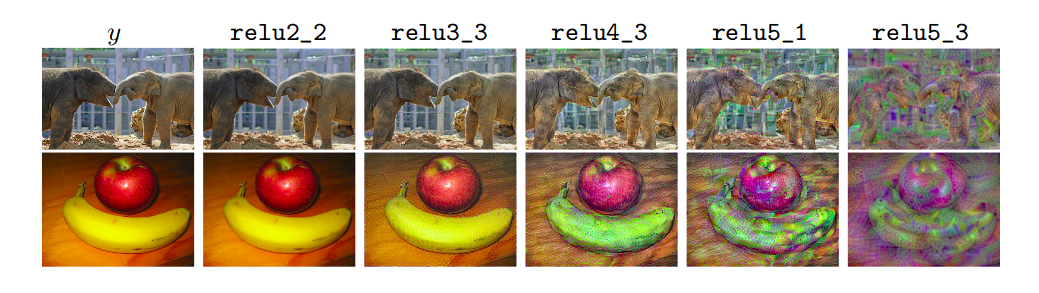
Now, the question appears how can we extract only content from content image and styles and textures from style image? Extract, this is where we saw CNNs excel at. We saw in our post on Visualizing CNNs that different layers extract different patterns like first layers in CNNs extract edges, second layers textures and as we go deep into further layers, high semantic concepts like faces, cars, text, etc are learned. Using these knowledge, we can see that we can use initial layers in CNN to extract styles and the content from high layers of CNN. In example below, we can see that if we reconstruct the original image from deeper layers we still preserve the high-level content of the original but lose the exact pixel information.
So, now we got general idea about how using pretrained CNNs can help in extracting patterns, textures and content. But how can we construct new image comprising of these two different representations? This question can be phrased as: how can we construct new image such that it’s content does not differ much from content image and also the new generated image’s style does not differ much in style and texture of style image. Now, the question can be easily solved by creating two loss function: content loss (\(\mathcal{L}_{content}\)) and style loss (\(\mathcal{L}_{style}\)).
\(\mathcal{L}_{content}(\mathbf{C}, \mathbf{P}) = 0\) which means we have a loss function which tends to 0 when it’s two input images (C and G) are very close to each other in terms of content, and grows as content deviate.
\(\mathcal{L}_{style}(\mathbf{S}, \mathbf{P}) = 0\) which tells how close in style two input images are to one another.
This style and content transfer problem is to find an image \(\mathbf{P}\) that differs as little as possible in terms of content from the content image \(\mathbf{C}\), while simultaneously differing as little as possible in terms of style from the style image \(\mathbf{S}\). In other words, we’d like to simultaneously minimize both the style and content losses.
\[\begin{aligned} \mathcal{L}_{total} = \alpha \mathcal{L}_{content} + \beta \mathcal{L}_{style} \end{aligned}\]\(\alpha\) and \(\beta\) are numbers that control how much we want to emphasize the content relative to style.
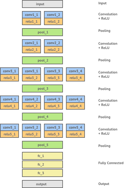
This shows similiarity to MNIST where we had a loss function defined, and then we ran optimizer to minimize the loss function. Similarly, Style Transfer is essentially an optimization problem where we minimize \(\mathcal{L}_{total}\) loss function. We still haven’t figured out as to what these respective loss functions represent(or are defined). To extract various features we use pretrained VGG16 as our base model (there is no standard as to which architecture to prefer). Here is the architecture,
- Content Loss(\(\mathcal{L}_{content}\))
Content Loss is the (scaled, squared) Euclidean distance between feature representations of the content and combination images. Given a chosen content layer \(\ell\), let \(\mathbf{F}^\ell\) be the feature map of our content image \(\mathbf{C}\) and \(\mathbf{H}^\ell\) the feature map of our generated pastiche image \(\mathbf{P}\). The content loss the will be,
\[\begin{aligned} \mathcal{L}_{content} = \frac{1}{2} \sum_{i, j}^{}(\mathbf{F}^\ell - \mathbf{H}^\ell)^2 \end{aligned}\]When the content representation of \(\mathbf{C}\) and \(\mathbf{P}\) are exactly the same this loss becomes 0.
- Style Loss(\(\mathcal{L}_{style}\))
This loss function is bit tricky. First we define something called Gram Matrix (\(\mathbf{G}\)). Gram Matrix extracts a representation of style by looking at the spatial correlation of the values within a given feature map. If the feature map is a matrix \(\mathbf{F}\), then each entry in the Gram matrix \(\mathbf{G}\) can be given by,
\[\begin{aligned} \mathbf{G}_{ij} = \sum_{k}^{}\mathbf{F}_{ik} \mathbf{F}_{jk} \end{aligned}\]
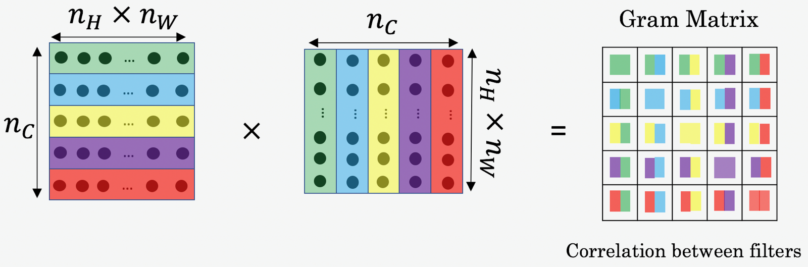
If we had two images whose feature maps at a given layer produced the same Gram matrix we would expect both images to have the same style, but not necessarily the same content.
Given a chosen style layer \(\ell\), the style loss is defined as the euclidean distance between the Gram matrix \(\mathbf{G}^\ell\) of the feature map of our style image \(\mathbf{S}\) and the Gram matrix \(\mathbf{A}^\ell\) of the feature map of our generated image \(\mathbf{P}\). When considering multiple style layers we can simply take the sum of the losses at each layer.
\[\begin{aligned} \mathcal{L}_{style} = \frac{1}{2} \sum_{\ell=0}^{L}(\mathbf{G}_{ij}^\ell - \mathbf{A}_{ij}^\ell)^2 \end{aligned}\]- Total variation loss(\(\mathcal{L}_{TV}\))
If you were to solve the optimisation problem with only the two loss terms we’ve introduced so far (style and content), we find that the output is quite noisy. We thus add another term, called the total variation loss (a regularisation term) that encourages spatial smoothness.
Now final loss function \(\mathcal{L}_{total}\),
\[\begin{aligned} \mathcal{L}_{total} = \alpha \mathcal{L}_{content} + \beta \mathcal{L}_{style} + \gamma \mathcal{L}_{TV} \end{aligned}\]
All pieces are in place. We run L-BFS or Adam Optimizer (L-BFS is preferred) as an optimizer to minimize the loss function.
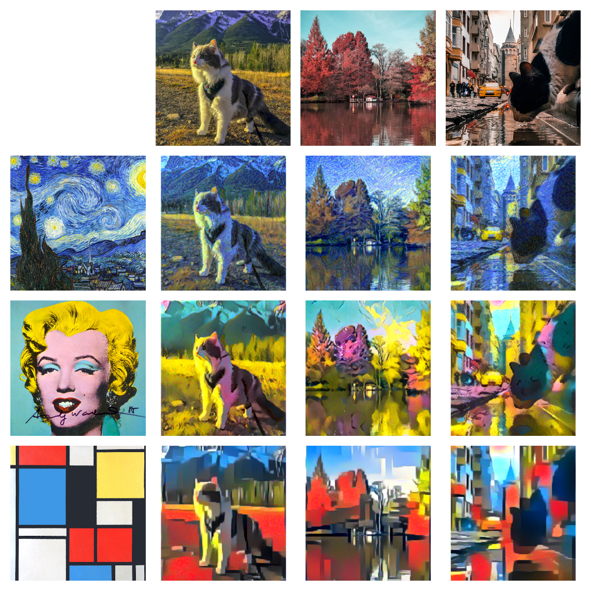
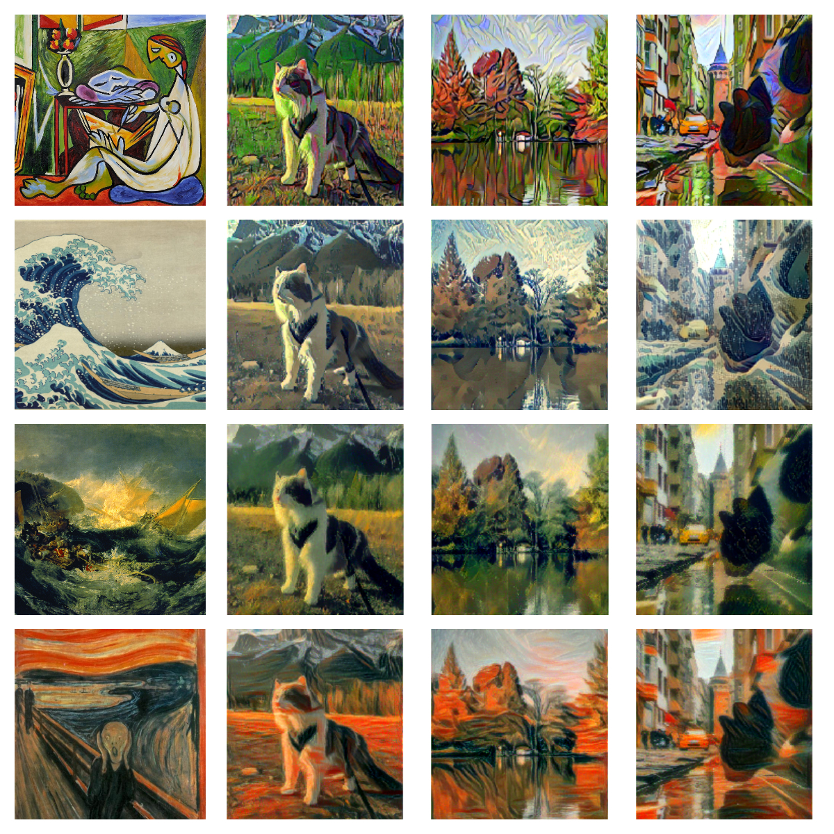
Et voilà ! the results,
Feed-forward Style Transfer
The drawback from above approach, other than being computuationally expensive is that we can style only one image at a time. For every other image pair (content, style), to produce styled image we have to run the algorithm again.
The paper, titled Perceptual Losses for Real-Time Style Transfer and Super-Resolution by Johnson et al, shows that it is possible to train a neural network to apply a single style to any given content image with a single forward pass through the network in real-time.
![]()
Architecture above, contains Image Transform Network and Loss Network.
- Image Transformation Network (ITN)
The architecture of Image Transfer Net as proposed by Johnson et al is shown in the diagram below.
![]()
It consists of 3 layers of Conv and ReLU non-linearity, 5 residual blocks, 3 transpose convolutional layers and finally a non-linear tanh layer which produces an output image.
- Loss Network
The loss network is used to calculate a loss between our generated output image and our desired content and style images. We calculate loss in the same way as the previous method, by evaluating the content representation of \(\mathbf{C}\) and the style representation of \(\mathbf{S}\) and taking the distance between these and the content and style representations of our output image \(\mathbf{P}\). These representations are calculated using pretrained VGG16 network.
The training regime consists of a input of content image batch, where ITN transforms it into pastiche images, loss network computes losses using pretrained VGG16 as done above, and calls backward on the final loss to update the ITN parameters. The loss network remains fixed during the training process. In their paper, Johnson et.al trained their network on the Microsoft COCO dataset - which is an object recognition dataset of 80,000 different images.
![]()
After training, generating style transfer for any content image takes less than 5 seconds to produce a styled version of given content image. This method is very fast and efficient than the one above as there is no retraining involved.
Here are some of the results,
Arbitrary neural artistic stylization network
We can spot one drawback from above method. We have to create seperate style transfer model for each new style image. Is there any method to allow real-time stylization using any content/style image pair? In other words, can we make a truly arbitrary neural style transfer network?
There are two methods:
- The work from Cornell University, proposed a new way to a simple yet effective approach to real time arbitrary style transfer without the restriction to a pre-defined set of style.
Authors propose a novel adaptive instance normalization (AdaIN) layer that aligns the mean and variance of the content features with those of the style features. Given a content input and a style input, AdaIN simply adjusts the mean and variance of the content input to match those of the style input.
The intuitive explaination of AdaIN from paper,
Let us consider a feature channel that detects brushstrokes of a certain style. A style image with this kind of strokes will produce a high average activation for this feature. The output produced by AdaIN will have the same high average activation for this feature, while preserving the spatial structure of the content image.
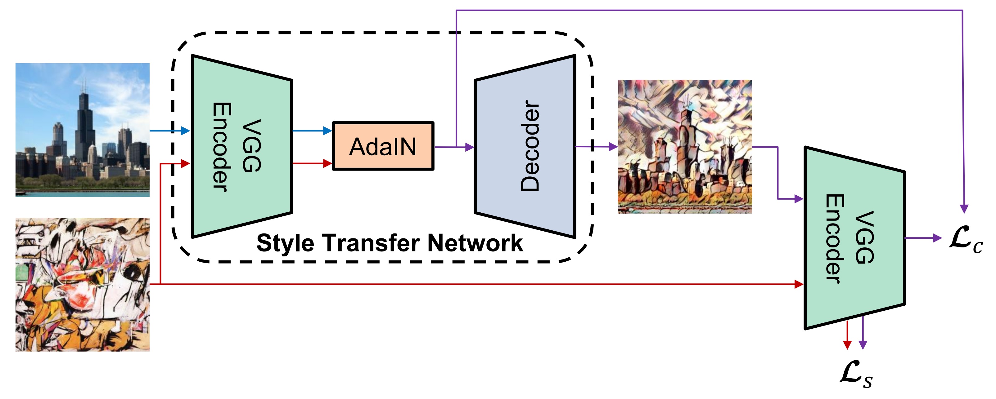
Style Transfer Network T takes a content image \(\mathbf{c}\) and an arbitart style image \(\mathbf{s}\) as inputs, it produces an output image that recombines the content of former and style of later. In encoder-decoder architecture, encoder \(\mathbf{f}\) which is fixed to first few layers (up to relu4_1) of pretrained VGG19 model. After enconding content and style images in features space, we feed both feature maps to an AdaIN layer that aligns the mean and variance of the content feature maps to those of the style feature maps, producing the target feature maps \(\mathbf{t}\) and a randomly initialized decoder is trained to map back \(\mathbf{t}\) to image space, generating stylized image.
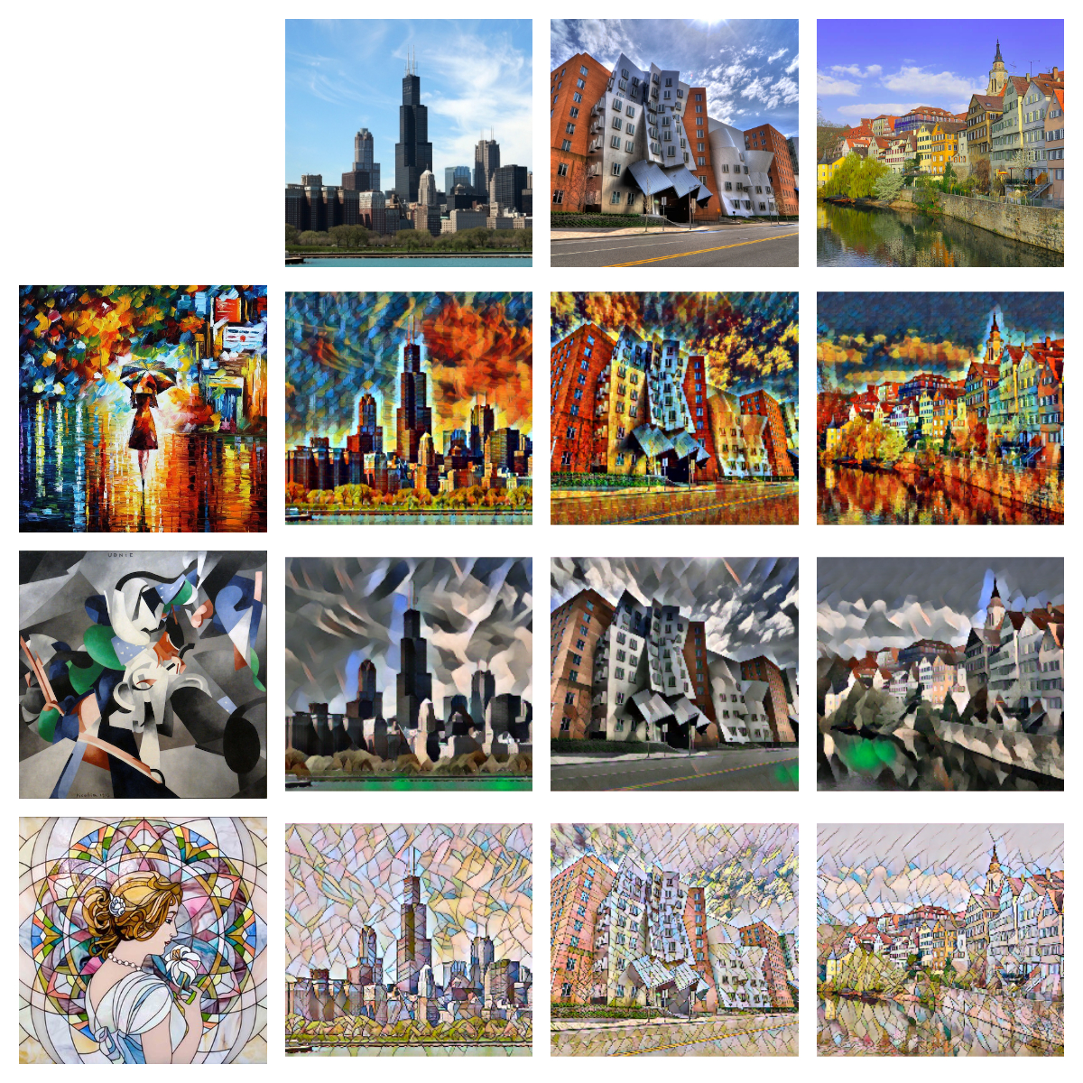
Here are some of the results from the paper on never seen style and content images,
- The work done at Google Brain where they overcome the drawback from above approach where the model can cover only a limited number of styles and cannot generalize well to an unseen style.
![]()
The style prediction network P(·) predicts an embedding vector \(\vec{S}\) from an input style image, which supplies a set of normalization constants for the style transfer network. The style transfer network transforms the photograph into a stylized representation. The content and style losses are derived from the distance in representational space of the VGG image classification network.
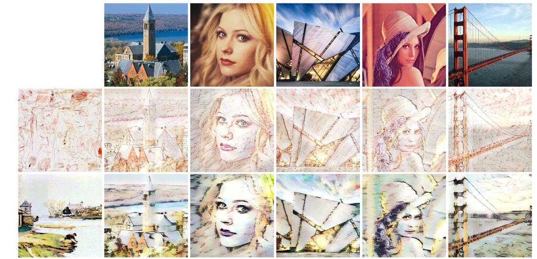
Here are some of the results borrowed from the paper,
![]()
This methods generalizes fairly to unobserved styles and content images.
Random Fact: Elmyr de Hory gained world-wide fame by forging thousands of pieces of artwork and selling them to art dealers and museums.
So young padwan, wasn’t it truly magical? Magic of Style Transfer . Similarly, in next post we will work on another cool application, Mystery of Object Detection .
Happy Learning!
Note: Caveats on terminology
Power of Transfer Learning - Transfer Learning
Power of Visualize CNN - Visualize CNN
Master Picasso - Pablo Picasso
Magic of Style Transfer - Neural Style Transfer
Mystery of Object Detection - Object Detection
ConvNets - Convolution Neural Networks
neurons - unit
cost function - loss or objective function
Further Reading
A Neural Algorithm of Artistic Style
Perceptual Losses for Real-Time Style Transfer and Super-Resolution
Supplementary Material for Forward-feed network
Arbitrary Style Transfer in Real-time with Adaptive Instance Normalization
A Learned Representation for Artistic Style
Exploring the structure of a real-time, arbitrary neural artistic stylization network
PyImageSearch: Neural Style Transfer OpenCV
How Does Batch Normalization Help Optimization?
Footnotes and Credits
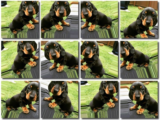
Sample style transfer example of dog
NOTE
Questions, comments, other feedback? E-mail the author